
Euler’s Number. The name is evocative. Leonhard Euler was one of the greatest Mathematicians and certainly one of the most prolific. As was typical in his time, Euler was a polymath, also making contributions to Astronomy, Engineering, Optics and what we would now call Physics. He produced deep results in a range of Mathematical fields and was innovative in both his ideas and terminology; being the first to introduce the fundamental concept of a function, to use the modern notation of trigonometric functions and to employ the Greek letter 
“Lisez Euler, lisez Euler, c’est notre maître à tous.” [1]
So if a number is named after Euler, then it is likely to be pretty important [2]. This is indeed the case, Euler’s Number is probably the most important number in Mathematics and I aim to give a flavour of why in this brief article. In order to do this, I need to lay some groundwork and some of this will be in areas that Euler himself advanced: functions, limits and differential calculus. But first some background.
Hail to e blithe constant [3]

Euler’s number is written as 


Non-terminating means that the numbers in the decimal representation of 
My recollection from school [4] was that
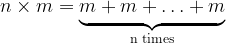
Let’s start with something even more familiar, multiplication. This is nothing bar repeated addition. So:

or symmetrically:

More generally, for two numbers 

or again symmetrically:

Of course the 


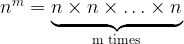
Exponentiation is the next step in this ladder [5]. This consists of repeated multiplication. So we have:
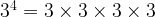
or more generally [6]:
In passing we will note some properties of exponentiation:

We can see how 

The other two identities are just as simply derived.


So (recalling that anything to the power zero is equal to one):


So:

There are even ways to raise digits to the power of Complex Numbers. However, now that we have some background on exponentiation under our belt, we can think about logarithms.

Logarithms are defined in terms of exponentiation. Consider:

We then define the logarithm of 


I.e. the logarithm of
Some examples include:

It should be noted that, though I am using Natural Numbers in the examples above, the definition of logarithms extends to fractions (aka Rational Numbers) and even – as we will see in a bit – numbers that cannot be expressed as fractions (aka Irrational Numbers)
We can now see why tables of logarithms used to be helpful. Supposing we wanted to multiply two largish numbers, say 


Then we have that:

and by

Algorithmically, we take the logarithms of each multiplicand, add these and then raise 10 to the power of the resulting number. In this case:

Which is a reasonable approximation to the actual answer, probably close enough for most practical purposes. As adding the logarithms is easier then multiplying two nine digit numbers (of course assuming that tables of logarithms have already been created), this approach historically saved labour.
Using both the definition of logarithms and the properties of exponents noted in 

Natural Logarithms are ones where the base is Euler’s number,

We then define the Natural Logarithm of 

I.e. the power to which we must raise
Well so far, so good, but we haven’t really got any insight as yet as to how Euler’s Number arises, or why it is so special. To obtain this we need to first spend some time contemplating functions, slopes and slopes of functions.
The Proper Function of Man [8]
Functions are one of the central concepts in Mathematics. They embody a relationship between a set of inputs and a set of outputs. A function can be thought of as a set of instructions on how to transform each input into each output. There is the proviso that each input has just one output. Thus the mapping between a function’s inputs and its outputs can be one-to-one or many-to-one, but never one-to-many (see below).

A function (typically denoted by one of 


This may be read as “a function
We can also write more concisely:

To take a few examples, we have:

Here we can see that the function is one-to-one, each output comes from only one input. Output 

| Aside:
We may in passing have also discovered the concept of the inverse of a function here and also stumbled across the fact that this only exists for one-to-one functions. The inverse of a function
This also means that In our example where |
 is a second function, labeled
  which “undoes” the transformation enacted by
  then
then  .
. 
 .
. then
then  .
.Let’s instead consider a different function (which we can also label

and:

If we revisit our previous examples, we have:

This time, we can see that the function is many-to-one, for example 
So far, we have looked at discrete inputs and outputs [11] If we keep the same recipe for our function, but change the input and output sets to both be the Real Numbers(

 = x^2")

Not only are the input and output numbers continuous [12], the line generated by the function is smooth, i.e. it has no sudden changes in direction. We will be coming back to this concept of smoothness very shortly.
So far I have covered functions that are powers of 

After this very brief introduction to functions, we hopefully understand them enough to move on to the next concept, slopes, or more properly gradients.
Why is a Blotter like a Lazy Dog?

The joke is rather dated (our writing tools have changed over the years), but:
A blotter is an ink-lined plane
An inclined plane is a slope up
A slow pup is a lazy dog– Anonymous
Here we will consider slopes up and indeed down and tie this to some of the earlier work in the article.
The road sign above provides a starting point and also the suggestion that gradients are ratios. Let’s start with a very simple example, where a “hill” is 5 miles long and has a rise of half a mile [13]; this is shown in the left-hand diagram below (please note that vertical distances have been exaggerated to aid clarity):

The gradient of the left hand slope is defined as how much height is gained divided by how much distance it takes to gain this height. In our example we have:

As our slope up is a straight line, the gradient is the same at any point. If we drew smaller triangles anywhere on our “hill”, the numerator and denominator of our gradient equation would change, but their ratio would remain constant. By way of contrast, consider the slope up in the right-hand diagram. Here we can see that the gradient changes as we go up. However, the average gradient is still the overall distance climbed divided by the overall horizontal distance covered. So in our example, the average gradient of both hills is the same [14].
| Aside:
The definition of gradient above should have some bells ringing from another area, Trigonometry. Let’s pause for a brief refresher on the basics of this. Consider a generic right-angled triangle as in the figure below:
Here the bottom left-hand angle has a value of 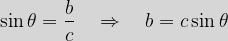
We can see that the definition of |

 , the hypotenuse has length
  , the adjacent side has length
  and the opposite side has a length of
  . We then have the following definitions:
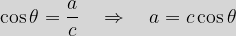
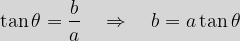
 is the same as that of gradient above.
Now let’s consider just the first two miles of the climb for both of our examples as follows (the segment highlighted in red below):

We can see that – consistent with our observation about smaller triangles above – the gradient of the left-hand “hill” is:

However that of the right-hand “hill” is:

While the average gradient of both climbs is the same, the local details of gradient differ.
What if, instead of looking at the gradient across some subset of the five mile climb on the right, we wanted to assess the steepness of the slope at various points. How would we go about this?
Well using the smaller triangles (the ones with a base of 2 miles) above suggests one approach. Supposing we wanted to know the slope of our right-hand “hill” at the 2 mile mark. Well we could construct a triangle whose base started on the “hill” at this point and stretched a little way to the right, say half a mile (or 880 yards [15]). If we zoom in, this might look like the following (again recall that vertical distances have been exaggerated in the diagram):

Our measurement of the gradient of this triangle is as follows:
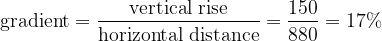
This seems like a decent estimate of the slope at 2 miles, but we could improve on it. What if we made the triangle smaller, so that its base was a quarter of a mile, or 100 yards, or 1 yard, or an inch. Intuitively it would seem that the smaller the triangle, the closer its slope would be to the actual gradient two miles into the climb. Indeed it would seem evident that if a certain level of precision in measuring the gradient was required, this could be achieved simply by drawing a small enough triangle.
The last paragraph may have seemed a little hand-wavy, but it is actually based on rigorous Mathematics. Once more this was an area to which Euler contributed strongly, the concept of limits.
The introductory part of this section is adapted from my book on Group Theory and Particle Physics, Glimpses of Symmetry [16]
In antiquity, Zeno of Elea propounded a number of paradoxes to do with motion. Here I am going to conflate two of them [17], but hopefully offer a simplification at the same time.

Consider an arrow being loosed towards a target. My simplification of Zeno’s argument – contrary to all experience of the physical world – is that it will never get there. The argument is as follows:
- In order to reach the target, the arrow must first cover half of the distance. Leaving half the distance to be traversed.
- Next it must cover half of the remaining distance, or a quarter of the total distance. Leaving a quarter of the distance to be traversed.
- Next it must cover half of the remaining distance, or an eighth of the total distance. Leaving an eighth of the distance to be traversed.
- And so on…
Because this process can be extended indefinitely, the arrow will always be short of the target. The distance it is short by will decrease rapidly of course, but there will always be a small distance still to be covered.
Therefore the arrow will never reach the target.
There is actually no paradox here and the theory of limits deals with any messiness quite nicely. Again Euler was a major figure in this area of Mathematics. To introduce it, let’s consider the distance remaining to travel in the above example. This forms a sequence as follows:
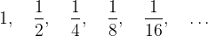
If we say that 

What happens to
| Opponent’s Number | Your Choice of  |
 |
| 0.1 | 4 | 0.0625 |
| 0.01 | 7 | 0.0078125 |
| 0.001 | 10 | 0.0009765625 |
It is probably evident that we will alway have the upper hand over our opponent. Indeed if we generalise by saying that the number they pick is denoted by 

(of course if 

So all we need to do to win our game is to pick 
In situations like this, where 

This can be read as “the limit of
The sense is that, if we can get arbitrarily close to a given value (in this case 0) by taking a large enough term in the sequence, then as the sequence wends its way to infinity, it actually reaches the given value, rather than just approaching it. Although this is not a very rigorous way of putting things Mathematically, we are sort of saying:

| Aside:
We formalise this result in exactly the way we established in our game above. We say:  If and only if, for any  That is however small a number is selected we can find a value of If we want to be more general, then if our sequence is  If and only if, for any Again the sense is that as |
 , we can find a value of
  we see that this assertion is true.
 then:
then:
 tends to
 Before closing this introduction to limits, we will cover just one more concept. If the distance remaining to be covered in our version of Zeno’s paradox is the infinite sequence we have been working with above, the distance that has been covered is instead an infinite series. Infinite series involve adding terms, the ones in this case are:
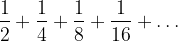
Using the notation that Euler himself introduced, we can write this as:

which can be read as “the sum of 
Formally, in terms of limits, what this means is:
The term on the right of the equals sign is called a partial sum. It captures the first
A corollary of the limit we established for the sequence

This is – in a nutshell – why motion is actually possible.
Having developed quite a bit of Mathematical machinery, much of it due to Euler himself, in the next two sections, we will begin to combine these concepts, first by considering the gradient of a function.
The introductory part of this section is also adapted from my book on Group Theory and Particle Physics, Glimpses of Symmetry [20]
In the section on gradients, we explored a way to find the slope of a “hill” at a given point using smaller and smaller triangles to increase precision. Some similarity between this process and the work we have just covered about limits is probably evident. Let’s drop our discussion of “hills” and be clear that what we want to be able to do is to determine the gradient of functions at specific points (we can think about drawing these functions on graph paper and measuring their slopes). Indeed, if our function is 


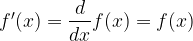
The function
While
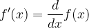
We read this as “the derivative of
Alternatively, if we set 

Similarly, we read this as “the derivative of
If we go back to our previous approach of drawing small triangles, but apply this to a function, 

Using our previous definition of gradient and considering the red triangle above, we have our estimate of the slope at point

Further as we shrink the size of

Let’s use this approach on a function we met earlier,

But:

So:
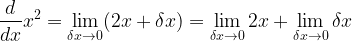
As, rather obviously, 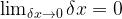

We can use similar arguments to show more generically that:
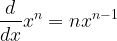 , where
I.e. to get the derivative of 

| Aside:
We have defined the process of differentiation of a function, 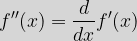 If we want to write this in terms of our initial function, then: 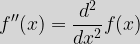 We can similarly form higher order derivatives such as |
 , to produce its derivative,
  . As
. As  , or indeed
  for the
  derivative. These can have a variety of physical meanings.
 Rather than providing many other examples of the derivatives of functions, it is time to cut to the chase and ask a question about differentiation that will lead us to our ultimate goal.

A we mentioned when introducing the topic, a function 
This second example is germane as – all other things being equal [24] – the number of bacteria at a future point is determined by how many there are now. This is because most bacteria reproduce by binary fission; each cell splits in two and so the number of bacteria doubles with each new generation. So if we have 
In an idealised situation, we would have the following number of bacteria at each successive generation:

Numerically, we have:

We can see that the rate of growth of the culture is dependent on its size, the bigger it is, the faster it grows. Putting this Mathematically, the derivative of the function giving us the population is dependent on the population itself, or 

Returning to our idealised state, we could rewrite the number of bacteria over time as:

E. coli split as frequently as every 20 minutes. If we took our time input as being chunks of 20 minutes, then we could form a rough formula as follows:

Where 

We seem to have created a function involving exponentiation, more on this shortly.
But now let’s abandon our bacteria before they engulf us and instead ask a more generic question. Can we find a function
That is a function whose derivative is precisely the function itself (or equivalently, the slope at a point is the value of the function at the same point)?
Well there are any number of ways that we could approach this, let’s just try some things out in a naive manner. I’ll take as a starting place our observation above that:
We can form a table using this result as follows:


A pattern appears here, the derivative of a function on one row is a multiple of the function on the previous row. Let’s look at what happens when we differentiate the terms we have in the table above put together in an expression:

Well that’s an interesting result. The derivative is close to the initial expression, but with all terms moving one place to the right.There is certainly a relationship between 
- The coefficients of each term (the numbers we multiply each power of
in the second one.
- We have lost our
term and so
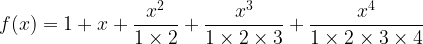
Can we fix these issues? Well to address the first point, we could try modifying our expression to be:
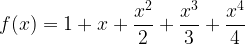
What happens when we differentiate this? Well we get:

At first sight, all seems good. However, having modified the definition of
What is the derivative of this?
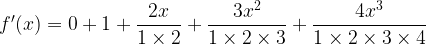
Cancelling out the same terms in each numerator and denominator, we get:
Which, if we drop the initial
Before moving on to address our second difficulty, a note about numbers like 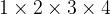

and more generally:

Using this notation (and noting that 
So what about our missing 
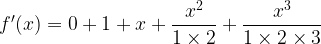
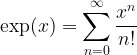
Well the concept of an infinite series as explored above comes to the rescue. Instead of the expression for

or using Euler’s summation notation:

We then have [27]:

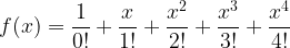
So we have constructed at least one function 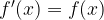
The choice of 
These equalities were proved directly by Euler again, though both Newton and Leibniz had come up with less direct and more convoluted proofs in the 1600s.
We call 
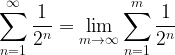
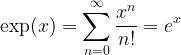
If we consider the value of 
Here we return to the beginning with a formula that expresses Euler’s Number as an infinite sum. Sometimes this is where people start to learn about
There are many other things to be said about
I will close by again reemphasising the self-referential manner in which The Exponential Function and Euler’s Number arise. As in several areas of Mathematics, self-reference leads to the emergence of interesting features. Also some of the apparatus we have developed allows the Exponential Function to be applied to many different Mathematical objects. We have mentioned Complex Numbers above, we can even do things like raising Euler’s Number to the power of a matrix [30]. In developing theories relating to the Exponential Function, as is much of the rest of his work, Euler opened up new Mathematical vistas, terrain which intrepid Mathematicians explore to this very day. I hope in this piece that I have given some flavour of his unique vision.
Acknowledgements
The following people’s input is acknowledged:
- Carey G. Butler, for pointing out a number of typographical errors.
- JohnKathy Mapp, who noticed that I was starting many of my summations at
was what it should have been.
- John S. Garavelli, who noticed I was erroneously using a
in equation
above, when a
- Caleb Fitzgerald, who pointed out a glitch in one of my examples of logarithms.
- Jonathan Baker, who pointed out an error in equation (3).
- Paul Macey, who straightened out my many-to-one and one-to-many text, which had got twisted.
Of course any [other] errors and omissions remain the responsibility of the author.
Notes
| [1] |
Read Euler, read Euler, he is the master of us all. |
| [2] |
Euler has the distinction of having a second number also named after him. The other is the Euler–Mascheroni constant. |
| [3] |
Sorry Percy :-o. |
| [4] |
Many years ago and so perhaps not to be relied upon 100%. |
| [5] |
The one after exponentiation is called tetration. It consists of repeated exponentiation, but this is outside of the scope of this article. |
| [6] |
Here we note that, unlike multiplication,  is not in general the same as is not in general the same as  . E.g. . E.g.  and and  . . |
| [7] |
In Pure Mathematics, the assumption is made that if  is used with no explicit base, then the base is and the meaning is Natural Logarithm. In other disciplines (and many scientific calculators), the formulation is used with no explicit base, then the base is and the meaning is Natural Logarithm. In other disciplines (and many scientific calculators), the formulation  is used instead. is used instead. |
| [8] |
I’m sure Jack London meant to add “or Woman”. |
| [9] |
gets used almost as much as in Mathematics. |
| [10] |
A point here is that while the output set is , the function only maps to values greater than or equal to zero (any negative number is mapped to a positive one). There is a term for the subset of the output range that a function covers, but we won’t be going in to this today. |
| [11] |
A set like the Integers is called discrete because there are gaps between its members, indeed there are an infinite number of values between any two Integers, say and  . If there are no gaps, the set is instead called continuous. . If there are no gaps, the set is instead called continuous. |
| [12] |
I.e. with no gaps in them, see Note 11 above. |
| [13] |
The units are immaterial, kilometres would have worked just as well, or cubits for that matter. We will drop units soon enough in what follows. |
| [14] |
Of course it is average gradient that appears on road signs as hills are seldom nice straight lines. |
| [15] |
Recall that there are 1,760 yards in a mile. |
| [16] |
Specifically a section in Chapter 21 – SU(3) and the Meaning of Lie. |
| [17] |
The first relates to Achilles and a Tortoise having a race, where the Tortoise has a head start; by the time Achilles has reached the Tortoise’s staring point, the Tortoise has moved – an so on. This paradox relates to fractions of distance covered, but is more complicated than is strictly necessary to make the point. The second paradox relates to an arrow in flight; arguing that at any instant in time, the arrow occupies a point, so therefore it cannot be moving. This paradox is more to do with the nature of time as it pertains to motion. Here I have blended the two to make what I think is a simpler example. |
| [18] |
It makes the format of the generic term easier to start with zero. |
| [18] |
It makes the format of the generic term easier to start with zero. |
| [19] |
Here  stands for the modulus of , which is effectively its absolute size. That is stands for the modulus of , which is effectively its absolute size. That is  . . |
| [20] |
Specifically a section in Chapter 20 – Power to Truth, which shares the same name. Any chance to reference a Smiths song is of course welcome. |
| [21] |
We can do this if the original function, is both continuous and smooth. Smooth has a specific technical meaning, which we won’t get into here. The general sense is not a million miles from the day-to-day meaning of the word. |
| [22] |
Somewhat sadly, schoolchildren are generally taught the rule before being shown why it works. |
| [23] |
Assuming that is smooth of course. We spoke before about smooth functions. In Mathematical terms, a smooth function is one that you can differentiate as many times as you want (possibly reaching 0 of course). |
| [24] |
Nutrients, space to grow, cells being immortal etc. |
| [25] |
We could of course rely upon our generic formula for the derivative, but if a function is equal to a constant, here 1, then it is a horizontal straight line when plotted on a graph. As with real hills, the gradient of a level line is zero. |
| [26] |
Again, we can see this result directly without recourse to our generic formula. If  then the graph of is a straight line going up from the origin at 45°. The slope of such a line is a constant one as each increase in the horizontal axis is matched by the same increase in the vertical axis. then the graph of is a straight line going up from the origin at 45°. The slope of such a line is a constant one as each increase in the horizontal axis is matched by the same increase in the vertical axis. |
| [27] |
We are able to make the last step in this chain of equalities for the same reason that we could drop in earlier expressions, namely:
For
we have 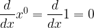 which can also be dropped allowing our sum to start from  |
| [28] |
The other, and perhaps less interesting, starting point is of course compound interest. |
| [29] |
With apologies to Pierre de Fermat of course. |
| [30] |
See a section of Glimpses of Symmetry, Chapter 20 – Power to Truth. |
|
Text & Images: © Peter James Thomas 2018. |
