< ρℝεν

|

ℂσητεητs

|

ℕεχτ >

“I admire the elegance of your method of computation; it must be nice to ride through these fields upon the horse of true mathematics while the like of us have to make our way laboriously on foot.” – Albert Einstein, in correspondence with Tullio Levi-Civita

Author’s Note This book is currently a work-in-progress. In case you stumble across it, please note that a number of Chapters are either incomplete or, in some cases, not yet started. The Chapter you are currently viewing falls into these categories. Expect content to be provided here in coming weeks and months.

It seems a long time since we defined the generic element of SU(3)’s smaller sibling, SU(2); this was back in Chapter 14. When later defining SU(3), I commented that characterising its elements would not be simple. It is towards this goal that we have been travelling over the last few Chapters, though the scenery out of the window has also been of general interest and general importance. The first part of this Chapter will consider what a generic element of SU(3) looks like. The second – and longer – part will describe Sophus Lie’s motivations in creating Lie Groups and Lie Algebras, covering more what they actually are and why they are of relevance in Physics as well as other areas.
 
 
SU(3) Unmasked

At the beginning of Chapter 15, we provided a formal definition of SU(3) as follows:

SU(3) is the set of 3 × 3 unitary matrices which also have a determinant of 1. We can write this as follows:

Where a_ij ∈ ℂ and det(A) means the determinant of matrix A.

Our task is to describe a generic element of S(3) and to do so, we will leverage its relationship with the Lie Algebra su(3). We met this back in Chapter 18 and it can be described as follows:

su(3) is the Real Vector Space of 3 × 3 Skew-Hermitian matrices whose trace is zero, with the Lie Bracket being the commutator. A generic element of su(3) is of the form:

Where a, b ∈ ℝ and α, β, δ ∈ ℂ.

Already, we can see that while it is hard to describe a generic element of SU(3) it is fairly easy to do so for su(3).

In addition, in Chapter 19, we noted that the following eight matrices form a basis for su(3) ^[1]:

If we label these σ₁, σ₂, … , σ₈, then – by definition – any element of su(3) is of the form:

a₁σ₁ + a₂σ₂ + … + a₈σ₈

For some a_i ∈ ℝ

However, in Chapter 20, we learnt that if we exponentiate each element of su(3), we get SU(3). Combining these two results, we can see that:

SU(3) = {e^{(a₁σ₁ + a₂σ₂ + … + a₈σ₈)}, such that a_i ∈ ℝ}

or equivalently:

SU(3) = {e^a₁σ₁ e^a₂σ₂ … e^a₈σ₈, such that a_i ∈ ℝ}

Expression as a quadratic in S [Consider expression via Sylvester’s formula – https://en.wikipedia.org/wiki/Sylvester%27s_formula cf. https://arxiv.org/pdf/1508.00868.pdf ]

 
Putting a New Spin on Things

https://www.quora.com/What-is-the-significance-of-SU-3-in-physics

https://www.quora.com/How-does-U-1-x-SU-2-x-SU-3-represent-the-Standard-Model

Note: For both some of the concepts and the general flow of material in this section and the next, I am indebted to Anthony Lee’s book Group Theory in a Nutshell for Physicists [2].

Back in Chapter 6 we spent time talking about rotations and reflections in 2D Euclidean Space and met the 2D Orthogonal and Special Orthogonal Groups, O(2) and SO(2), that consist of such transformations. In Chapter 15, we introduced the concept of the dot product of two vectors in Euclidean Space, noting that:

If v = (v_x, v_y) and u = (u_x, u_y) then we can define the dot product of v and u equivalently as:

v.u = |v||u| cos θ          (A)

where θ is the angle between the two vectors, or:

v.u = v_xu_x + v_yu_y          (B)

Note: With respect to definition (B), it is worth noting that if we think of both v and u as 2 × 1 matrices (as we did in Chapter 17) then we are unable to multiply these (you can only multiply n × m and m × p matrices), but that if we were to turn v round to make it a 1 × 2 matrix, then matrix multiplication is not only allowed, it gives us the same result as the dot product. We have applied the term transpose to date only to square matrices, but we can also describe this turning round of v as replacing it with vT as follows: We will come back to this approach a little later.

For now, we also recall that SO(2), which covers only rotations, is made up of matrices as follows:

The physical meaning of the angle φ is that the matrix rotates objects in Euclidean Space (or equivalently Euclidean Space itself) by an angle φ around the origin.

Note: Back in Chapter 13 we demonstrated that the Circle Group, T, the Unitary Group of degree 1, U(1), and SO(2) were all isomorphic, i.e. essentially the same Group. We spent some time in Chapter 19 looking at how to create the Tangent Space of U(1), so – at least to some extent – we will be covering old ground in this Chapter. The treatment will be very different here, but it is worth also recalling the connection with the earlier work.

Let’s use the label M_φ to denote a generic matrix in SO(2), one that represents a rotation by φ.

One might be tempted to ask, what happens to our dot product if we apply M_φ to both of our vectors, i.e. if we rotate them by φ?

We then need to consider:

v′ = M_φv

and

u′ = M_φu

Writing these out long-hand we get:

So what about the dot product of the two transformed vectors? If we first focus on definition (B), we can see that:

v′.u′ = (cos φ v_x – sin φ v_y)(cos φ u_x – sin φ u_y) + (sin φ v_x + cos φ v_y)(sin φ u_x + cos φ u_y)

Multiplying out the brackets we get:

v′.u′ = cos² φ v_xu_x – cos φ sin φ v_xu_y – sin φ cos φ v_yu_x + sin² φ v_yu_y + sin² φ v_xu_x + sin φ cos φ v_xu_y + cos φ sin φ v_yu_x + cos² φ v_yu_t

The terms in red and the terms in blue cancel one another so we have:

v′.u′ = cos² φ v_xu_x + sin² φ v_yu_y + sin² φ v_xu_x + cos² φ v_yu_t

Or:

v′.u′ = (cos² φ + sin² φ) v_xu_x + (cos² φ + sin² φ) v_yu_y

Noting that, by Pythagoras, cos² x + sin² x = 1, this means that:

v′.u′ = v_xu_x + v_yu_y = v.u

So the dot product is unchanged by multiplying by an element of SO(2), or equivalently by rotating both vectors. We can say that the dot product is invariant under rotation.

A brief consideration of definition (A) would lead us to this conclusion even quicker as clearly a rotation through and angle of φ changes neither the length of either vector, nor the angle between them.

If we go back to our matrix multiplication notation, we have shown that:

v^Tu = v′^Tu′

However, if we worked the other way and instead insisted that the dot product – as per definition (B), which involves no explicit trigonometry – is preserved by a transformation encapsulated in some matrix M_φ, where the subscript φ could be viewed as a whim of labelling, then what could we deduce about M_φ?

Well if we start with the requirement that:

v^Tu = v′^Tu′          (1)

We also have:

v′ = M_φv          (2)

and

u′ = M_φu          (3)

A property of transposes is that (AB)^T = B^TA^T, where it should be noted that the order of multiplication is reversed. So if we take the transpose of both sides of (2), then we have:

v′^T = v^TM_φ^T          (4)

Using (4) to substitute for v′^T and (3) to substitute for u′ in (1), we get:

v^Tu = v′^Tu′ = v^TM_φ^TM_φu

or:

v^Tu = v^T(M_φ^TM_φ)u

Which obviously only works if we have:

M_φ^TM_φ = I          (5)

So we have ascertained that the transpose of M_φ must also be its inverse. At this point some bells may be ringing from our definitions of U(2) and SU(2) back in Chapter 14, albeit that these were based on Complex 2 × 2 matrices and here we are dealing with Real ones.

If we take the determinant of both sides of (5), we have:

det(M_φ^TM_φ) = det(I)          (6)

In Chapter 17 we mentioned that det(A^T) = det(A), to this we can add the property that det(AB) = det(A)det(B), applying both of these to (6), we get:

det(M_φ^TM_φ) = det(M_φ^T)det(M_φ) = det(M_φ)det(M_φ) = 1

Which of course means that:

det(M_φ)² = 1, or det(M_φ) = ±1          (7)

The combination of (5) and (7) actually provides the more normal definition of O(n) and SO(n), the Orthogonal and Special Orthogonal Groups of degree n. O(n) is those matrices where just (5) holds, SO(n) is those where, in addition, det(M) = 1, i.e. just rotations (if the determinant is – 1, then these are reflections). So we have arrived at these two groups simply by considering restrictions on the dot product, ignoring the trigonometric approach we employed in Chapter 6.

Can we apply this approach more broadly? We can indeed, but first let’s explore Marius Sophus Lie’s central idea, which relates to how we might decompose transformations.
 
 
The Journey of a Thousand Miles… ^[3]

In antiquity, Zeno of Elea propounded a number of paradoxes to do with motion. Here I am going to conflate two of them ^[4], but hopefully offer a simplification at the same time.

Consider an arrow being loosed towards a target. My simplification of Zeno’s argument – contrary to all experience of the physical world – is that it will never get there. The argument is as follows:

1. In order to reach the target, the arrow must first cover half of the distance. Leaving half the distance to be traversed.
    
2. Next it must cover half of the remaining distance, or a quarter of the total distance. Leaving a quarter of the distance to be traversed.
    
3. Next it must cover half of the remaining distance, or an eighth of the total distance. Leaving an eighth of the distance to be traversed.
    
4. And so on…

Because this process can be extended indefinitely, the arrow will always be short of the target. The distance it is short by will decrease rapidly of course, but there will always be a small distance still to be covered.

Therefore the arrow will never reach the target.

The theory of limits of infinite series deals nicely with the above, which is actually no paradox at all. As we saw in Chapter 20, we have:

So, happily for all involved (save maybe for the gentleman standing on the right above), motion is possible.

As well as laying Zeno’s mind to rest, results like the one above suggest that we can decompose motion into smaller and smaller pieces, indeed maybe an infinite number of pieces, while still having the concept make sense. The movement of the arrow can be split into an infinite number of infinitely small (infinitesimal) segments and all is still well. It is to a certain extent on this observation that Sophus Lie’s insight rests.

Rather than arrows, let’s think about some transformation, maybe a rotation by 60° (π/6 radians) counter-clockwise ^[5]. How is this achieved? Well instead of one rotation of 60° we could do two rotations of 30° each, or 8 rotations of 7.5° (see the diagram below), or 60 rotations of 1° each, or 600 rotations of 0.1° each.

Indeed we could pick arbitrarily small fractions of the total rotation and – so long as we performed enough of these – still get to our final destination. If all of these mini-rotations are the same, then we can characterise the whole process by just the first of them. E.g. when we had 60 mini-rotations, understanding what a rotation of 1° does enables us to understand the 60° rotation.

Our mini-transformations can still be captured by some matrix, but if the transformation is infinitesimal, so will the matrix be. If we consider a rotation matrix M_δφ where the angle δφ is infinitesimal, then the transformation it enacts will be very close to the identity matrix plus some infinitesimal matrix. We could write that:

M_δφ ≈ I + E

where E is an infinitesimal matrix.

Indeed for a infinitesimal rotation, we can drop the approximation and simply use an equals sign:

M_δφ = I + E

What happens if we apply the restriction we developed above, that M_δφM_δφ^T = I? Well we then have:

I = M_δφM_δφ^T = (I + E)(I + E)^T

By the same properties of transposes we used above, this becomes:

I = M_δφM_δφ^T = (I + E)(I + E^T)

Multiplying out we get:

I = M_δφδM_φ^T = I² + IE^T + EI + EE^T

But if E is infinitesimal, EE^T will be smaller still and so can be ignored, giving us:

I = M_δφM_δφ^T = I + E^T + E

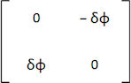
Which means that E = – E^T. We call matrices fulfilling such a property skew-symmetric (again we may begin to hear echoes of work we did in Chapter 18 ^[6]). Any 2 × 2 skew-symmetric matrix will be of the form ^[7]:

Equivalently, we can say that the matrix on the right-hand side is a basis for what is evidently a 1D Vector Space of such matrices; we can derive any element from it by multiplying by a scalar.

If we want to better define what our rotation matrix, M_δφ, looks like, a helpful approach is to see what it does to the elements of a basis; in this case a basis of 2D Euclidean Space. As any vector in Euclidean Space can be described in terms of basis elements ^[8], seeing what happens to them under a transformation obviously yields insight about the transformation itself. For this reason, let’s now consider the action of M_δφ on the basis of 2D Euclidean Space we last met in Chapter 16: {1_x, 1_y}, where 1_x = (1, 0) and 1_y = (0, 1).

We could approach this question just using linear algebra ^[9], however a geometric figure is probably going to make things clearer in the first instance; we still need no trigonometry here. Given this, we can capture the action of M_δφ on these two vectors in the following diagram:

We can see that a rotation of δφ moves 1_x to 1_x′ and 1_y to 1_y′. Both vectors move along the unit circle centered at the origin and – if we assume that δφ is expressed in radians – then as per Chapter 11, we can see that the length of the red and blue arcs that this movement inscribes are also both equal to δφ ^[10].

However, if the angle δφ is small enough, then straight red and blue lines pointing respectively straight up from (1, 0) and straight to the left of (0, 1) are almost equal to the length of the red and blue arcs. We can say that the length of these straight lines is approximately δφ. If the angle δφ shrinks further to become infinitesimal, we can drop the approximation and state that the micro-rotation moves the tips of the two basis vectors respectively δφ up and δφ to the left. We thus have:

(1, 0) ↦ (1, δφ)

(0, 1) ↦ (- δφ, 1)

In matrix form, we can write this as:

Returning to our previous finding, we can see that this is indeed of the form:

M_δφ = I + E

where E is an skew-symmetric infinitesimal matrix of the form:

Indeed we can see that the scalar, λ, we used to describe E above is just δφ.

If we refer back to the partial table of Lie Algebras we presented at the start of Chapter 20, we can also see that the set of all such matrices nothing other than the Lie Algebra so(2) ^[11].

So, by considering infinitesimal transformations that approximate to part of our original Group transformations (and equal them in aggregate), we have [technically] done the equivalent of forming the tangent space to SO(2) at its identity element (the 2 × 2 identity matrix) and [less technically] achieved a change in perspective from the original Group to a structure susceptible to treatment under liner algebra; we have linearised SO(2).

Shortly we will look at how the concept of exponentiation for reconstituting SO(2) from so(2) arises, but first let’s deal with a remaining characteristic of a Lie Algebra, its Lie Bracket.

[Physical meaning of the commutator]

Having drilled down into infinitesimal characterisations of continuous transformations, particularly the rotations in the Group SO(2), let’s try to put the pieces together. Suppose we have some element of SO(2), a matrix, M_φ, that generates a rotation by φ, where φ is not an infinitesimal angle, but something more quotidian like 90°, or 135° (π/2 or 3π/4 radians). We have already seen that we can break the overall rotation of φ degrees down into smaller elements; let’s chose to split it into n equal elements, each one a rotation of φ/n. Now each of these smaller rotations is identical and each one is enacted by the same matrix, M_(φ/n). To reconstitute M_φ, we simply need to multiply all of n identical mini-rotations, i.e.:

M_φ = M_(φ/n) × M_(φ/n) × … × M_(φ/n)

Where there are n terms in the multiplication on the right-hand side.

We can write this more economically as:

M_φ = M_(φ/n)ⁿ

Now when n becomes large, clearly φ/n becomes small and we already uncovered a way to describe M_(φ/n) for small angles, we can state this as:

M_(φ/n) = (I + E)

Where E is equal to:

If we use E₀ to denote our basis vector (i.e. the matrix on the right with entries {0, – 1, 1, 0}), then E = (φ/n)E₀ and we have:

M_φ = (I + φE₀/n)ⁿ

The above formula may bring to mind the compound interest example we covered in a footnote to Chapter 20. In this earlier example, as we calculated interest over more numerous, but shorter, time periods, Euler’s constant, e, emerged. What happens as n gets bigger (and indeed tends to infinity) in the above expression? Well we have:

So we can see that:

M_φ = e^φE₀

M_φ ∈ SO(2) and φE₀ ∈ so(2), so we have a mapping, χ, as follows:

χ : so(2) ↦ SO(2) : φE₀ ↦e^φE₀

As flagged earlier, this is effectively a repeat of the result pertaining to u(1) and U(1) that we presented in last Chapter. However, the path we have taken above probably gives a more visceral sense of how a Lie Group, here SO(2), can be reconstituted ^[12] by exponentiating members of its corresponding Lie Algebra, here so(2). We also hopefully begin to see why the mysterious process of exponentiating works. It is a natural byproduct of reversing the process by which a Group element, representing a continuous transformation, is decomposed into an infinite number of infinitesimal transformations, each of which is a member of the related Lie Algebra.

The process we have just gone through explains both how the concept of the Lie (or infinitesimal) Algebra of a Lie Group arises and why Lie Groups and their Algebras are connected in the way we described in Chapter 20.

[To be completed

Consider: https://en.wikipedia.org/wiki/Root_system

Consider: https://en.wikipedia.org/wiki/Quark_model%5D

Concepts Introduced in this Chapter TBC TBC. TBC TBC.

Groups Discovered in this Chapter TBC TBC. TBC TBC.

< ρℝεν

|

ℂσητεητs

|

ℕεχτ >

Chapter 21 – Notes

[1]	I could have used the Gell-Mann matrices (also see Chapter 19) instead, which might have been more appropriate in a book at least tangentially related to Particle Physics. However I would then have had to add and i in the exponential function as well.
[2]	See the Acknowledgements.
[3]	“… begins with a single step.” – Lao Tzu in Tao Te Ching circa 4th Century BCE Though both the author and date of the book remain questionable.
[4]	The first relates to Achilles and a Tortoise having a race, where the Tortoise has a head start; by the time Achilles has reached the Tortoise’s staring point, the Tortoise has moved – an so on. This paradox relates to fractions of distance covered, but is more complicated than is strictly necessary to make the point. The second paradox relates to an arrow in flight; arguing that at any instant in time, the arrow occupies a point, so therefore it cannot be moving. This paradox is more to do with the nature of time as it pertains to motion. Here I have blended the two to make what I think is a simpler example.
[5]	The same argument applies to any other sort of transformation, so long as it is continuous (i.e. it is susceptible to being split into smaller and smaller parts). A counterexample is that a reflection is not a continuous transformation, there are no intermediate stages.
[6]	Although – as again we were working with Complex matrices in Chapter 18, the concept was Skew-Hermitian rather than Skew-symmetric. If a Skew-Hermitian matrix has entries restricted to ℝ, then it becomes Skew-symmetric.
[7]	The elements of the main diagonal don’t change and so must be equal to their own negative. The only way that a = – a is if a = 0.
[8]	The definition of a basis.
[9]	The ability to employ linear algebra – as opposed to either geometry or trigonometry – is indeed a motivation here, especially in higher dimensional Vector Spaces. Linear algebra will, in general, be a simpler approach.
[10]	This is how radians are defined.
[11]	As mentioned in the partial table of Lie Groups and Lie Algebras, the same set also constitutes o(2), i.e. o(2) = so(2), whereas SO(2) ⊂ O(2). The reason is that O(2)\SO(2) is precisely reflections, which – unlike rotations – are discontinuous transformations and so cannot be decomposed into a large number of small parts the way we can with rotations. This also implies that o(2) only partially generates O(2).
[12]	Or rather that it can, in general, at least be partially reconstituted. For so(2) and SO(2) – and indeed for so(n) and SO(n) – the reconstitution is complete.

Text: © Peter James Thomas 2016-17. Images: © Peter James Thomas 2016-17, unless stated otherwise. Published under a Creative Commons Attribution 4.0 International License.