< ρℝεν

|

ℂσητεητs

|

ℕεχτ >

“Just as you can write a book about mountains without requiring your readers to climb one, you can write a book about equations without requiring your readers to solve one. Still, readers of a book about mountains probably won’t understand it if they have never seen a mountain…” – Ian Stewart, in Why Beauty is Truth: The History of Symmetry

 
Turning the Tables
 
Having previously introduced the pivotal Mathematical concept of matrices and worked out how to add and multiply them, this Chapter considers some of their other important properties; how they can transform objects and even transform space itself. These are properties to which we will return in later Chapters of this book. For now, in order to further explore the effects of matrix multiplication, let’s start by going back to the type of grid we defined in the particle example at the beginning of the previous Chapter, but this time we’ll focus matrices which contain location information.

If we define a rectangle whose vertices are:

A: x = 2, y = 2

B: x = 2, y = 4

C: x = 6, y = 4

D: x = 6, y = 2

We can view each x and y paring as a row in a 4 × 2 matrix as follows ^[1]:

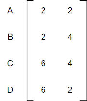
(NB the letter labels are just to make clear which row represents which vertex, they are not part of the actual matrix)

Below we list out what happens when we operate on this rectangle with some modified versions of our identity matrix:

We can plot the results of these on the same type of “graph paper” as we used in our previous example and the result is as follows:

A cursory glance shows that multiplying by each of these matrices is equivalent to respectively:

reflecting using a mirror lying along the x axis

reflecting using a mirror lying along the y axis

carrying each of the above reflections one after another

There is some sense in which we started with the somewhat numeric concept of matrices and are now finding ourselves back in the physical world of reflections we explored back in Chapter 3. Let’s continue pushing ahead and consider multiplying by some new matrices ^[2] as follows:

Again we can plot the outcome in the same way we did for the last batch of transformations:

So once more we can ascribe a physical interpretation to these multiplications, specifically:

Rotate by 90° clockwise

Rotate by 180° clockwise, which is the same as the reflect across the x axis and then the y axis transformation we saw above

Rotate by 270° clockwise

Direction of Travel I’d like to pause to note something important at this point. In the above, if A is the matrix which holds the vertices of our rectangle and R is one of the rotation matrices which we have been considering, then we have been looking at the effect of post-multiplying A by R, namely AR. We could of course have instead looked at RA, however – based on the rules of multiplication that we explained in the last Chapter – we would have to reformulate A as a 2 × 4 matrix instead of the 4 × 2 one we have used above. If we do this, we get: It is immediately apparent that two of the three answers are now different (recall that matrix multiplication is not commutative). We can also chart these rotations as follows: Doing this makes it apparent that the difference is the direction of the rotation, in this case anti-clockwise as opposed to clockwise. The physical meanings this time are: Rotate by 90° anticlockwise Rotate by 180° anticlockwise, this is the rotation which is the same – clearly rotating 180° clockwise is the same as rotating 180° anticlockwise Rotate by 270° anticlockwise We will be doing some pre-multiplying later in this Chapter and it is important to remember the distinction.

To return to our original reflections and rotations, if we replaced our rectangle with a triangle, centred this so that the axes from vertices to the mid-points of the opposite side all intersected at the origin and modified our reflectional and rotational matrices (see the box below) to relate to 120° rather than 90° ^[3], then we would have a set of matrices which are isomorphic to the Dihedral Group of degree 3, the symmetry group of a triangle as covered in Chapter 3. Indeed we don’t actually need the triangle, we can simply use the matrices to move the entire 2D space around and the transformations will again be isomorphic to the Dihedral Group of degree 3. The linkages between numbers and physical reality run very deep!
 
 
In the following box, I’ll look at rotations using matrices in more depth and try to genericise the results we have demonstrated above. While an understanding of the methods that I’ll use to construct more general rotational matrices is optional (hence the box), there are some strong relations to other, more complex, matrices we will meet later in Chapter 13. For this reason I recommend that readers at least skim the contents of the following box.

Generic Gyrations After learning about the above matrices, which turn elements of the 2D coordinate space through multiples of 90°, it might occur to the reader to ask whether there is a way create rotations with different angles (for example the 120° I mention above). We’ll explore this question in this box. The rotations and reflections we have considered to date consist of finite lists, we can write all of them down. When a finite number of matrices act on objects (in this case by rotating the through a finite number of angles, e.g. 0°, 90°, 180° and 270°) we call these transformations discrete. There are only a certain number of predetermined angles through which an object can be rotated and there are gaps (in the above case gaps of 90°) between each of these. In this box, we are going to start talking about infinite sets of matrices which can rotate an object by any angle. These are called continuous transformations as there no finite list of angles to which their action is restricted and therefore also no gaps between the angles through which objects can be rotated. It is somewhat like the difference between the Integers and the Real Numbers; the former has gaps in between, the latter does not (though of course here the Integers are also of infinite size). One way of considering a set of continuous rotational transformations is to note that, for any two angles and their associated rotation matrices, we can find an angle between them and create its related rotation matrix and so on ad infinitum. In order to begin we need to recall a little Trigonometry. Let’s start by considering a right-angled triangle as shown below: Here the bottom left-hand angle has a value of θ, the hypotenuse has length c, the adjacent side has length a and the opposite side has a length of b. We then have the following definitions: sin θ = b/c cos θ = a/c If we consider a generic point in the same two dimensional space we have been using to look at rotations and reflections, then this can be written as (a,b) where a is the x coordinate (the distance along the x-axis) and b is the y coordinate (the distance along the y-axis). We can draw a line from the origin (0,0) to (a,b) and drop a vertical from (a,b) to the x-axis. This forms a right-angled triangle and then we have the following: If θ is the angle between the line going to (a,b) and the x-axis, then the same trigonometric equalities we defined above hold. If we rearrange them slightly, we can say: a = c cos θ and b = c sin θ So we could replace (a,b) with (c cos θ, c sin θ). This observation is going to help us as we think about rotations. Suppose we want to rotate our point anti-clockwise around the origin by an angle φ, ending up at a new location (a’,b’). By this I mean that the distance between the point and the origin remains constant, so such a rotation would bring the point closer to the y-axis, but move it further from the x-axis. If, in the same way we did above, we construct a second right-angled triangle with (a’,b’) as a top vertex, then its hypotenuse will still have a length of c, but its other two sides will have new lengths, a’ and b’. This can be seen below: Can we work out a way to represent such a generic rotation as a matrix? Well we can start by noting that the left bottom angle of the second triangle is given by θ + φ. Again we can calculate the lengths of its two shorter sides in terms of the hypotenuse and the angle it makes with the x-axis, so: a’ = c cos(θ + φ) and b’ = c sin(θ + φ) Two well-known trigonometric identities deal with the sums of angles as follows: cos(A + B) = cos A × cos B – sin A × sin B and sin(A + B) = cos A × sin B + sin A × cos B We can use these to rewrite our expressions for a’ and b’ as follows: a’ = c cos θ × cos φ – c sin θ × sin φ and b’ = c cos θ × sin φ + c sin θ × cos φ (I’ll generally – but probably not consistently – drop the × from expressions like this going forward. ) But from our original triangle, we already know that a = c cos θ and b = c sin θ. If we substitute these values back into the above we get: a’ = a cos φ – b sin φ and b’ = a sin φ + b cos φ So a becomes a cos φ – b sin φ and b becomes a sin φ + b cos φ. How can we effect this mapping? If we consider (a,b) as a 2 × 1 matrix then we need a 2 × 2 matrix which does the following: A little thought (and recalling how matrix multiplication works) yields the following result:

The 2 × 2 matrices describing rotations in a 2 dimensional space which we derived in the box above form a Group called the Special Orthogonal Group of degree 2, or SO(2). This is defined as follows:

In order to verify this statement, we need to go through our customary tick-list:

1. Closure

   First of all an appeal to intuition. If we rotate by an angle θ and then by an angle φ the result is the same as rotating by the combined angle, θ + φ.

   Taking the approach of multiplying matrices we see that:

   

   If we go back to the trigonometric identities for cos(A + B) and sin(A + B) that we cited in the box, then we can instead write:

   

   As the final matrix is clearly of the same form as the rest of SO(2), this establishes closure more formally.
    

2. Identity

   Obviously we know the matrix which is the Identity for 2 × 2 matrices, that is:

   

   The question is whether this is a member of SO(2). If we pick a value of φ equal to 0° then we get:

   

   So we have an Idenity ∈ SO(2).
    

3. Inverse

   Once more let’s start with an appeal to intuition. If we rotate by φ anti-clockwise, then rotating by φ clockwise (equivalently rotating by -φ anti-clockwise) will bring us back to where we started.

   More formally, we can represent this by multiplying the following two matrices (and employing the same trick with sin(A+B) and cos(A+B) that we used above):

   

   This shows that any element of SO(2) has an inverse, which is also in SO(2).

   In Chapter 5 we noted that, in order to have an inverse, a matrix must have a non-zero determinant. From the generic definition of the matrices making up SO(2), we can see that the determinant of any of them is in fact -sin²φ -cos²φ = -1. So our non-zero requirement is also met. We’ll reference determinants of these and simmilar matrices again later in this Chapter.
    

4. Associativity

   This holds because we have already proved that matrix multiplication is associative.

We will be coming across another Group isomorphic to SO(2) in Chapter 13, indeed it will be one of the Groups central to this book, the Unitary Group of degree 1, U(1).
 
 
From Dihedral to Orthogonal

When we looked at the symmetries of shapes, such as the equilateral triangle, we formed a Group, the Dihedral Group, by combining the rotations and reflections. Having genericised discrete rotations of an n-gon into continuous rotations above, can we do the same for reflections? Again the answer is yes and the necessary mathematics is covered in the next box. As with all boxes, if you are more interested in the destination than the journey, you can skip forward to where the main text picks up again. However, as with the details of how we constructed matrices carrying out general rotations, some familiarity with how we approach generating reflections will come in useful later.

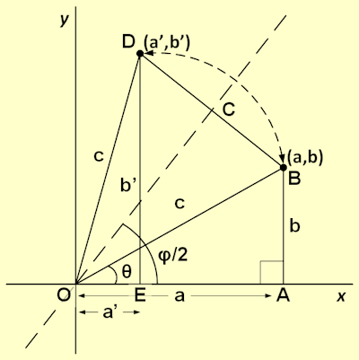
Moveable Mirrors First of all let’s think about the set of reflections that we examined at the beginning of this Chapter. They invoved “mirrors” lying on the x- and y-axes. In order to consider reflections through any angle, what we need to do is to construct a generic “miror” passing through the origin, (0,0), and at any given angle to the x-axis. To do this, we’ll adopt an approach similar to the one we used for continuous rotations earlier in this Chapter. First of all, let’s define a generic point, (a,b), which makes an angle θ with the x-axis (see the first diagram in the previous box). As before, let’s assume that the hypotenuse of the right-angled triangle that this makes with the x-axis has a length of c. Recall that, as in the previous box, we have: a = c cos θ and b = c sin θ Now let’s draw a line of reflection through the origin and making an angle φ with the x-axis. Actually this will work out a lot more neatly if instead we consider the mirror being set at an angle of φ/2 to the x-axis. φ is an arbitrary angle and so φ/2 is equally arbitrary and this change in definition makes no difference. These choices of angles are shown below: The reason for this rather artificial-seeming choice of definition for φ will probably become apparent as we further elaborate on this diagram below and start to create some equations based on it. What we want to do is to construct the reflection of (a,b) in this general “mirror”. If we label this new point (a’,b’) then once more we can start to construct some right-angled triangles as follows (rather than resorting to leaden prose, I’ll let the image do the talking): In particular. If we want to work out the angle that (a’,b’) subtends with the x-axis, then this has three components as follows: ∠AOB = θ ∠BOC = (φ/2) – θ ∠COD = ∠BOC (noting that △BOD is isosceles) Adding all of the above up, we get this angle being: 2((φ/2) – θ) + θ = φ – θ Here of course the reason for using φ/2 as our angle becomes apparent. So we can see that the position of (a’,b’) is given by: a’ = c cos(φ – θ) and b’ = c sin(φ – θ) Going back to our identities for cos(A+B) and sin(A+B), there are equivalents for cos(A – B) and sin(A – B) which are as follows: cos(A – B) = cos A cos B + sin A sin B and sin(A – B) = sin A cos B – cos A sin B Using these we can determine the values of a’ and b’ as follows: a’ = c cos θ cos φ + c sin θ sin φ and a’ = c cos θ sin φ – c sin θ cos φ If we use the formulae we established for a and b above, we get: a’ = a cos φ + b sin φ and b’ = a sin φ – b cos φ 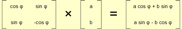So once again we are looking for a 2 × 2 matrix which fits the following equation: It can fairly readily be seen that the way to construct this is as follows:

One of the motivations for looking at a continuous definition of reflections (matching the continuous definition of rotations we earlier established) was to combine both to see if we can construct a continuous equivalent of the discrete Dihedral Groups. Having put all of this effort into defining rotations of arbitrary angle and reflections in a line of equally arbitrary angle, it would be rather a shame if the resulting structure was not a Group. Happily we are spared this fate and what we create by combining the reflections and rotations we have created is the Orthogonal Group of degree 2, O(2). This is the set of all 2 × 2 Orthogonal Matrices. Orthogonal Groups form an infinite family where O(n) is the set of n × n Orthogonal Matrices.

In Chapter 13 we will meet a type of matrix called Unitary matrices. Orthogonal Matrices are strongly related to these. To define orthogonality, we need to first introduce an operation that can be carried out on matrices, this is called transposition.

Transposition involves keeping the diagonal of a matrix constant, but swapping the diagonally opposite entries to the south west and north east of these. So for a 2 × 2 matrix A, where:

Its transpose, written as A^T, is:

Similarly for a 3 × 3 matrix, B, we have:

With this definition under our belt, we can define an Orthogonal Matrix, A, as one for which:

AA^T = A^TA = 1 (where here 1 denotes the n × n identity matrix)

or equivalently

A^-1 = A^T

Then the Orthogonal Group of degree n is defined as follows:

That is the set of n × n Orthogonal Matrices.

It’s pretty straightforward to show that our infinite sets of both 2 × 2 rotation and reflection matrices are orthogonal as follows:

I am not going to prove here that all orthogonal 2 × 2 matrices are either reflections or rotations (though I will prove something analogous to this for Unitary Matrices in Chapter 13), however this second result is also true, so we can also say for at least O(2):

Let’s assume this definition and use it to validate that O(2) is indeed a Group:

1. Closure

   We already know that the rotational matrices are closed under multiplication. So we need to check what happens if we combine two reflections and if we combine a reflection and a rotation. Intuition suggests that a reflection followed by another reflection should equate to a rotation of some angle and that a reflection followed by a rotation should equate to a rotation through some other angle ^[4]. Let’s test these hypotheses:

   

   Which shows that our intuition was correct and O(2) is closed.
    

2. Identity

   This is the normal 2 × 2 identity matrix, which we have already shown is part of SO(2) and thus part of O(2).
    

3. Inverses

   We established that inverses of rotations existed when looking at SO(2). Obviously the inverse of a reflection is the same reflection. So we have inverses.
    

4. Associativity

   Again this is a property of matrix multiplication.

So O(2) (using our reflections and rotations definition) is indeed a Group.

Before closing this Chapter, it is worth pointing out something about the determinants of members of O(2). It may be recalled from the last Chapter that the determinant of a generic 2 × 2 matrix {a, b}{c, d} is simply ad – bc. Looking at our definitions of rotations and reflections above:

For a rotation matrix A, det(A) = cos²φ + sin²φ = 1

For a reflection matrix B, det(B) = -cos²φ – sin²φ = -1

In particular for all matrices M ∈ O(2), |det(M)| = 1 (where |x| is the size – ignoring sign – of x). This is something we will return to again in Chapter 13.
 
 
We have seen that multiplying by different matrices can achieve a lot of different results. There are effects beyond the ones that I have covered above. Matrix multiplication can grow or shrink shapes, or skew and deform them in interesting ways ^[5]. Many more pages could be covered in discussing the properties of matrices and indeed we will be coming back to this subject later in the text. However, for now I want to keep the end in mind and we now have one more element in place in our quest to explain unitary and special unitary groups. One of the next planks will fall into place in the next chapter. Having plotted the impact of matrix multiplication on shapes in a two dimensional space, we will now look at a rather different, if analogous, two dimensional space. This one will have a more numerical flavour and consists of the Complex Numbers.
 

Concepts Introduced in this Chapter Reflectional Matrices These can be used to reflect objects in any line passing through the origin of a n-dimensional space. Variants of the 2 × 2 identity matrix (obtained by changing the sign of one or both of the 1s) reflect objects across the x- or y-axes of two dimensional space. Continuous reflectional matrices reflect objects by in a line of any given angle. Rotational Matrices These can be used to rotate objects around an origin of a n-dimensional space. Variants of the 2 × 2 identity matrix (obtained by changing the sign of both of the 1s, or by having the 1s on the south east / north west diagonal, instead of the normal north east / south west) rotate objects by multiples of 90° in two dimensional space. Continuous rotational matrices rotate objects by any given angle. Pre- and Post Multiplication If pre-multiplying by a rotational matrix, R (i.e. RA, for some matrix A), results an anticlockwise rotation of angle φ then post-multiplying by R (i.e. AR for some matrix A) will result in a clockwise rotation of angle φ. Transpose The transpose of a matrix is obtained by keeping all entries on the north east / south west diagonal fixed, but getting all elements off this diagonal to swap places with the corresponding element on the opposite side of the diagonal. The transpose of a matrix A is denoted by AT. Orthogonal Matrix An n × n matrix (with entries in the Real Numbers) for which AAT = ATA = 1 (where here 1 denotes the n × n identity matrix). Equivalently, A-1 = AT. Orthogonal Determinant The determinant of an n × n Orthogonal Matrix is either 1 or -1, so |det(A)| = 1 for all A ∈ O(n).

Groups Discovered in this Chapter SO(n) The Special Orthogonal Group of degree n. This infinite Group is of all continuous rotations around the origin, or equivalently all n × n orthogonal matrices whose determinant is equal to -1. For SO(2) the 2 × 2 matrices are of the form: O(n) The Orthogonal Group of degree n. This infinite Group is of all continuous rotations around the origin and all reflections in lines passing through the origin, or equivalently all n × n orthogonal matrices. For O(2) the 2 × 2 matrices are of the form:

< ρℝεν

|

ℂσητεητs

|

ℕεχτ >

 
Chapter 6 – Notes

[1]	We could equally view it as a 4 × 2 matrix, we’d just have to do the multiplications the other way round instead.
[2]	And one which we have met already.
[3]	This area is covered in greater detail in the next box of this Chapter.
[4]	We covered these types of combinations of rotations and reflections in Chapter 3 when considering the Group of symmetries of an equilateral triangle, the Dihedral Group of degree 3.
[5]	A few of these are covered in Chapter 17.

Text: © Peter James Thomas 2016-18. Images: © Peter James Thomas 2016-17, unless stated otherwise. Published under a Creative Commons Attribution 4.0 International License.