This article is both adapted and extended from a piece that I originally wrote on Q&A site Quora.com back in 2017.
 
 
As someone with a Mathematical background, I have spent long periods of my life working with numbers. There are many beautiful different types of these that can be constructed (or is that discovered?). The process starts with the first building blocks, the Counting Numbers, which are known more technically as the Natural Numbers. However our journey to discover the nature of numbers will take us into much less familiar territory. Along the way, I will attempt to introduce you to the most salient parts of the extensive Number Menagerie. My aim is to make the material as accessible as possible to a non-Mathematical audience. Inevitably there are formulae here, but I hope that I build things up in a way that can be followed by the able and engaged reader.

The types of numbers I cover are as follows, most of them are labelled with a capital letter in a Blackboard Bold font:

• Natural Numbers – denoted by
• Prime Numbers – oddly, given their importance, the Primes have no letter
• Integers –
• Rational Numbers –
• Real Numbers –
• Complex Numbers and Gaussian Integers – and
• Quaternions and Octonions – and

For each I have adopted a bullet-point style, which hopefully stresses the essential facts, rather than cocooning these in extraneous prose. Along the way a few additional explanations are included as asides in boxes. Let’s start by looking at the basic Counting Numbers mentioned above, the Natural Numbers.

 
Natural Numbers,

• These are the “counting numbers”, so:
   
  

   

  Aside: The notation indicates that what falls between the curly brackets is a set, a collection of things. All animals is a set, all cats is a subset of this. So here is a label for all the numbers listed between the curly brackets, including those hinted at by the

  Some people nowadays also include in this set, but I’m a traditionalist and would call this set non-negative Integers (see below).
   

• The above implies that the Natural Numbers go on for ever. There is no end to the Natural Numbers, or to put it another way, there is no biggest Natural Number.
   
• To see this, suppose on the contrary that the largest Natural Number is , then clearly is also a Natural Number and bigger than , a contradiction. If a statement leads to a contradiction in this manner, the statement itself must be false.
   
• We use the word infinity to describe sets like that go on for ever.
   
• As we will see soon, there are different magnitudes of infinity. The size of the Natural Numbers is labelled , pronounced Aleph Null. Any infinite set which has a size of is called Countably Infinite as we can use the Natural Numbers to count them (see An aside about Counting below).

 
Prime Numbers

• Prime numbers are Natural Numbers that have precisely two factors, themselves and 1.
   
• A factor of a Natural Number is one that divides it with no remainder. So is a factor of because . is not a factor of because the remainder when it is divided by is 1, .
   
• 1 is not a Prime because it has just one factor, 1.
   
• Prime Numbers are important for many reasons, notably because any Natural Number greater than can be expressed as a unique product of Prime Numbers (if you ignore the order in which they are multiplied). This is the Fundamental Theorem of Arithmetic.
   

  Aside: Here we going to introduce the symbol , which is used to denote that something is a member of a set, for example . may be read as “in”, “belongs to” or “is a member of”.

  The Fundamental Theorem of Arithmetic states that for any we can find Prime Numbers, (possibly with some repeats), such that .
   
  

  For a proof of this and some examples, see Glimpses of Symmetry, Chapter 8 – Simplicity.
   
• There are an infinite number of Primes as well. To see this, assume the contrary and that is a complete list of all Prime Numbers. Then construct the following number, . No number , which is greater than 1, divides , so this means than none of our list of Primes can divide . Therefore either has no prime divisors and so is prime itself, or it has some other prime divisor, say , which does not appear in our finite list. Either way a contradiction arises, so our assumption that the Primes were finite is erroneous.
   

  Aside: This proof is a modern recasting of the one originally devised by the eminent Greek Mathematician Euclid circa 300 BC.

• The Primes also have precisely the same size as the Natural Numbers, .

  Here we note one of the odd things about infinite sets, a subset can be as big as the whole set – in the same way the set of all even Natural Numbers is the same size as the size of the Natural Numbers – or, as Richard Feynman put it, “there are twice as many numbers as numbers”.

 
An aside about Counting

• Above we called the Natural Numbers the counting numbers, here let’s consider what counting actually means. When we say “Five little ducks went swimming one day” what we are actually doing is setting up a relationship between the set of ducks and the Natural Numbers.

  

  This may sound a bit esoteric, but if I say that what we do is to point at the first duck and say “one”, point at the second duck and say “two”, the third and say “three” and so on, then the process hopefully becomes a more familiar one.

  As this is a written article and not a vlog, I’m going to use some notation to describe this process. I will write to mean pointing at a duck (or something else) and saying “one”. Similarly I will write if I want to point at the second frog in a set. We will come back to this notation below when talking about both Integers and Real Numbers.

 
Integers,

• Here we extend the Natural Numbers by including and negative whole numbers (whole numbers is a bit of a fuzzy term, so I have, in general, excluded it from this article), so:
   
  .
   
• As with Natural Numbers and even Natural Numbers above, perhaps counterintuitively, there are the same number of Integers as Natural Numbers. Recalling our duck-centric notation, if we define to mean pointing at and saying “one” and as pointing at and saying “two”, then we can count the Integers like this: , , , , , , , , then we have matched each element of with each element of and thereby established that they are the same size.
   
• If we want to consider just negative integers , we use the symbol . is just the Natural Numbers again.

 
For more background on the Natural Numbers and Integers, see: Glimpses of Symmetry, Chapter 2 – What is a Group?

 
Rational Numbers,

• Rational Numbers are fractions both positive and negative, so numbers like:
   
  

   
  and so on.
   

• However, a loose definition of fractions would include that abomination, , which as every schoolchild learns is the work of the devil and to be avoided at all costs.
   
• It would also include, for example:
   
  

   
  which is probably not what any of us had in mind when using the term.
   

• A way to avoid such complications is to define in terms of the numerators and denominators of its elements as follows:
   
  

   

  Aside: Here we introduce some more notation. To date, we have generally been explicit (or at least indicative) about which numbers make up a set. Instead, what we have above is a sort of recipe for creating the members of a set, namely the Rational Numbers. The bit directly after the first curly bracket and before the vertical bar shows the general pattern of set members. The bit after the vertical bar and before the second curly bracket provides restrictions on the general pattern. The vertical bar itself can be read as “such that”. For example, consider the set . This is the even Natural Numbers; the set of numbers of format such that is a Natural Number. So our definition of the Rationals can similarly be read as “numbers consisting of a divided by b, such that a is an Integer and b is a Natural Number”.

   
  This definition alone is enough for me to argue that keeping zero free is worth it.
   

• Perhaps strange to say, there are no more Rational Numbers than Natural Numbers. If we create an array of the Rational numbers as follows:
   
  

   
  It may be readily seen that any Rational Number will appear in it somewhere. If we again use our convention that is pointing at and saying “one”, we can count the Rational Numbers by tracing a winding route through the array as follows:
   
  , , , , , , , , , ,
   
  The path we take looks like this:

  

• If (as shown above) we can count the Rationals (more formally if we can set up a mapping between the Natural Numbers and the Rational Numbers), then the Rationals are also Countably Infinite.

 
Real Numbers,

• 
   
  If we consider a line extending out from zero in both a positive and a negative direction, never ending on either side, the the Real Numbers are the inhabitants of this line.
   
• It might be thought that we have just effectively duplicated the definition of the Rational Numbers, but this is not the case. There are Real Numbers which are not Rationals. Indeed, in a sense, the vast majority of Real Numbers are not Rational.
   
• The canonical way to show this is by considering the radical . It can be shown relatively easily ^[1] that there are no two numbers and such that . Equivalently, is not a member of .
   
• is clearly a number, to ten decimal places it is equal to . However the decimal expansion of never actually ends and never settles down to any repeating pattern. This formulation leads to one of the most common ways of viewing Real Numbers as decimals and including those that go on for ever. We can then say:
   
  

   
   

  Aside: Above we use the symbol which indicates infinity. Where the context is counting to infinity – as it clearly is above – this means the version of infinity, i.e. the size of the set of Natural Numbers.

• Any Rational Number can also be expressed using this approach, but the numbers after the decimal point will settle down to a pattern, e.g.:
   
  

   
  or
   

  

   

• A Real Number that is not a Rational Number is called an Irrational Number (meaning “not a Rational” as opposed to “illogical”). The Mathematical notation applied to two sets and means: all elements in set that are not in set . So we can write the Irrational Numbers as . Irrational numbers – like – will never have their decimal expansion settle down to a repeating pattern.
   
• A final type of Real Number completes this menagerie. They too have a weird name, Transcendental Numbers. Irrational numbers like are the root of some polynomial equation ^[2] with Rational coefficients, in this case .
   

  Aside: A polynomial (meaning “many names”) is an equation of the form: Where the are constants, typically Integers or Rational Numbers, called coefficients and is the variable, or unknown; the thing that is to be found. The general idea is to find which number, or numbers, when substituted for result in a value of . The highest power of that appears is called the degree of the polynomial. Some polynomials of small degree have special names. Degree one polynomials (where the highest power is itself) are called linear. Degree three polynomials (where the highest power is ) are called cubics. Nestling in between these are polynomials of degree 2, or as every schoolchild is taught, quadratics. An example of a quadratic is the equation: Which can be factored into: Showing that it has the solutions and . For more complicated quadratics, the same schoolchildren are taught a standardised formula which yields the solution of , namely: The above indicates that, as in our simple example, there are two values of x that satisfy the quadratic equation, one is calculated using a in the formula, the other a instead. All quadratics have two solutions. In general, a polynomial of degree n will have n solutions (some of which may be repeated), these are often referred to as roots of the polynomial.

  Transcendental Numbers are Irrational Numbers that are not the root of any finite polynomial equation with Rational coefficients. The two best known Transcendentals are , most commonly defined as the ratio of a circle’s circumference to its diameter ^[3], and Euler’s Number, ^[4]. However, again Transcendentals are more common than non-Transcendental, Irrational Numbers, though not all have the special properties of and .

  Below we show each of , and on our Real Number line:
   
  
  

   
• Readers may have been getting the feeling that the size of all sets of numbers is the same as the Natural Numbers. Here we come across a counter-example. The size of the Real Numbers is actually larger than the Naturals, the Real Numbers are not countable. This result is derived from a famous proof by Georg Cantor. This runs as follows:
   
• First of all, let’s assume the opposite, that the number of Real Numbers (Rationals plus Irrationals) is countably infinite. To make our work easier, let’s just focus on the segment of the number line , you can easily generalise from here. So any Real Number in this interval can be written as , where the are digits in .
   
• If these numbers are countable, then we can (by definition and like with the little ducks above) set up a one-to-one correspondence between the Natural Numbers and the Real Numbers in this interval, something like:
   
  

   
  and so on (this is the essence of counting of course).
   

• Now consider the diagonal of this array (highlighted in bold above) and use this to create a new number as follows. Pick different from , different from , different from , and so on. Clearly this new number doesn’t appear anywhere on the original list, it is different from the first number in the first place after the decimal point, different from the second number in the second place after the decimal point and so on. So we have assumed that the Reals are countable and used this to create a Real Number which is not in the list of Real Numbers paired to the Natural Numbers, a contradiction. Therefore the Real Numbers cannot be countable.
   

  Aside: There are some technicalities to be considered in the above argument, for example and being precisely the same number, these have been elided here for the sake of clarity.

• It might be tempting to assume that the size of the Real Numbers is , i.e. the next biggest type of infinity. However, this opens a can of worms. The Real Numbers are sometimes also known as the continuum. The size of the continuum is denoted by and it may be shown that . The statement that is known as the continuum hypothesis. This margin is too small to contain ^[5] a full review of the continuum hypothesis and the reader is invited to research this elsewhere ^[6].

 
More background about both Rational and Real Numbers may be read in Glimpses of Symmetry, Chapter 4 – Rationality and Reality

 
Complex Numbers and Gaussian Integers, and
 
I attempted to provide a gentle introduction to the Complex Numbers in Glimpses of Symmetry, Chapter 7 – Imaginary Battleships and would recommend anyone unfamiliar with the area starting here. In this piece instead I will jump straight in.
 

• The Complex Numbers are an extension of the Real Numbers that we met above. The extension is achieved by introducing a new number, , which is defined as . The set of Complex Numbers is denoted by and the way that the extension works is by setting:
   
  

   
  As an aside, and are the same Complex Number, the order of multiplication is immaterial, I will probably swap between the two notations in places.
   

• The number is not an artificial one. In the section on Real Numbers, we saw how a non-rational number, , arose by considering the solutions (roots) of the quadratic equation, . The number arises in a similar way by considering the roots of a different quadratic, , or .
   
• A lot of people have problems accepting as a real (lowercase “r”, so no pun intended) number. This comes from confusion about the nature of numbers themselves. All numbers are abstract concepts. The reader may object saying that they know that they have 5 fingers (or little ducks). However what is happening here is that a relationship is being set up between a set of things (fingers) and another set (the Natural Numbers). The number is no more concrete than , it is just a convenient label we use because it is helpful to do so. The duck-centric diagram I provided above makes this explicit. The issue is that we do this so often and so unconsciously that it seems different to other abstractions like . What is important is not so much whether or not a number is “real”, in a sense none of them are, but rather whether or not it is well-defined and helpful.
   
• On the helpful side, of course the introduction of the Complex Numbers allows us to provide solutions to all finite polynomials, something we could not achieve with just the Reals. So there is one use. More broadly, many calculations in real-world areas, such as engineering, fluid dynamics or electronics, have Complex Numbers appear half way through and then magically disappear later in the workings, yielding a correct answer. If the step including the Complex Numbers was skipped, the answer could not be derived. They are also somewhat useful in Particle Physics, as covered in several chapters of Glimpses of Symmetry ^[7].
   
• Complex numbers of the form , or just , are called Imaginary Numbers. This somewhat problematic nomenclature is perhaps one reason why they can be viewed as mystical by some people.
   
• Having defined , we can state that , where is any positive Real Number.
   
• A Complex Number, , can be seen to have a Real part, , and an Imaginary part, . We write and . The Real and Imaginary parts are somewhat independent of each other, so if we add two Complex Numbers, we have which it may be seen is the same as, , or even more explicitly, , the result being obtained by adding the Real and Imaginary parts separately.
   
• Multiplication is a little more complicated. (by the definition of ). Which we can rearrange as, .
   
• For a Complex Number , an important concept is its conjugate, written which is obtained by changing the sign of just the Imaginary component, i.e. .
   
• The conjugate comes in useful when we want to divide Complex Numbers. Consider:
   
  

   
  If we multiply both top and bottom by the conjugate of , i.e. , we get:
   

  

   
  multiplying out both top and bottom we get:
   

  

   
  which we can write as:
   

  

   
  which is clearly another Complex Number (assuming one of and is non-zero, or equivalently ).
   

• Given the way that addition and multiplication work, one important way of visualising Complex Numbers is the Complex Plane, a coordinate system where the Real part of a Complex Number is plotted on the horizontal, or x-axis and the Imaginary part is plotted on the vertical, or y-axis as follows (note the position of the Complex Number ).

  

• It can be seen that taking the conjugate of a Complex Number is equivalent to reflecting it in the x-axis.

  

• We can use the Complex Plane and some basic Trigonometry to further our understanding of Complex Numbers.
   

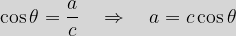
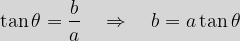
  Aside: Before going any further, let’s pause for a brief refresher on the basics of Trigonometry. Consider a generic right-angled triangle as in the figure below: Here the bottom left-hand angle has a value of , the hypotenuse has length , the adjacent side has length and the opposite side has a length of . We then have the following definitions: (the last purely for the sake of completeness).

• Now let’s construct a triangle by drawing a line from the origin of the Complex Plane (, or just ) to a Complex Number and dropping a perpendicular to the x-axis as follows (where is the angle that makes with the x-axis):

  

• First of all, we can define the size of , written as being the length of the line we have drawn. Using Pythagoras, we can see that . Then Trigonometry gives us and . So we can write .
   
• But now we can now recall Euler’s Formula ^[8] that . If we use this in the above, we can see that , so we have a way of expressing any Complex Number using the Exponential Function. The fact that the Exponential Function with a Complex argument is periodic (something also implicit in the link to and above) explains some of why Complex Numbers appear in the study of waves and things that rotate (see also Glimpses of Symmetry, Chapter11 – Root of the Problem and Chapter 13 – First Contact – U(1)).
   
• So far, we have been expanding out our number definitions, however we can move in the opposite direction. Let’s consider a subset of the Complex Numbers defined as follows:
   
  

   
  These are know as the Gaussian Integers, which are denoted by . In the Complex Plane, if you consider horizontal lines running through each of and vertical lines running through each of , then the Gaussian Integers appear at the intersections of these sets of lines. You can add, subtract, multiply and even divide (with remainder) Gaussian Integers. There is even the concept of prime Gaussian Integers.
   

• Finally, given that is essentially made of two copies of spliced together (again think the x- and y-axes), it might be thought that the size of is greater than the size of . Once more intuition lets us down. Actually the two numbers are equal. The slightly weird way that cardinalities of infinite sets (also known as transfinite numbers) work mean that: .

 
Quaternions and Octonions, and
 
The following section is adapted from a box entitled “The Sign of the Four” which appears at the end of Glimpses of Symmetry, Chapter 7 – Imaginary Battleships.

• So we defined the Complex Numbers in terms of the Real Numbers by introducing to get: . Maybe we could add just another element like , say . It turns out that this doesn’t really work, but if we take a further step and introduce a third new element, , then something wonderful happens, we have found the Quaternions, first discovered by Irish Mathematician William Hamilton in 1843.
   
• The set of Quaternions is denoted by in honour of Hamilton. It is defined as follows:
   
  

   

• We can use these definitions to form a table capturing how the various elements combine as follows:
   

  ×	i	j	k
  i	– 1	k	– j
  j	– k	– 1	i
  k	j	– i	– 1

• We can also fairly readily see that numbers in are well-behaved, you can add, subtract, multiply and divide them in ways analogous to what we have demonstrated for earlier in this article. One point to note however is that multiplication is not commutative ^[9] (i.e. ), indeed in general if are two distinct generators (i.e. each a different one of ) then , as may be seen in the table above.
   
• Of course a natural follow-on would be to wonder whether or not we can take this process of extending the concept of number further. There is one further extension, the Octonions, which unsurprisingly have eight generating elements analogous to the four for the Quaternions. However that is then it, there is no meaningful set of numbers with 16 generating elements or indeed any more. The reason is that we lose features of the number system along the way, the Quaternions are not commutative, the Octonions are not associative ^[10] – i.e. – and there is nothing much left to lose beyond this while retaining meaning as a number system.

 
More background about Complex Numbers and Quaternions may be read in Glimpses of Symmetry, Chapter 7 – Imaginary Battleships

 
Here we will stop our journey into the realms of Numbers. There are other towns and villages that we could have taken in along the way. We have not mentioned other number bases, such as Hexadecimals, or the Binary System; both of which are important in Computing. We could also start to put our numbers (of whatever sort) into tables with rows and columns, also known as matrices. Beyond these, Modular Numbers ^[11], p-adic Numbers and Hyperreal Numbers come to mind, as does the important area of Finite Fields. However hopefully the trip has still been a pleasant and stimulating one, albeit that we skipped on some esoterica.

It is a long and winding road from the Natural Numbers to the Octonions. I trust that I have been able to show that it is a navigable path and that there are some inherent properties shared by all the numbers we have looked at above; they can be added, they can be multiplied and so on. I also trust that I will have helped at least some readers to expand what they view as being a number. It is a big Mathematical Universe out there and, if my brief notes have whetted your appetite, there is a wealth of helpful material available at different levels of sophistication and just a quick Google away.
 
 

---

 
Acknowledgements

The following people’s input is acknowledged:

• John Heaver, who pointed out that The Fundamental Theorem of Arithmetic applies only to Natural Numbers greater than .

Of course any [other] errors and omissions remain the responsibility of the author.
 

Consider Supporting Us   Like all of the content on peterjamesthomas.com, this article is free. However, if you enjoyed reading it, you might consider helping to support the creation of new content by making a small contribution to defray our costs. Pay as much or as little as you want. Of course this is entirely optional. Peter James Thomas

 

<<	Glimpses of Symmetry	When I’m 65	>>
Part of the peterjamesthomas.com Maths and Science archive.

 
Notes

[1]	See a footnote to Glimpses of Symmetry, Chapter 4 – Rationality and Reality.
[2]	See a second footnote to Glimpses of Symmetry, Chapter 4 – Rationality and Reality.
[3]	However, also see More π in the sky – Quora.
[4]	See a section of Glimpses of Symmetry, Chapter 20 – Power to Truth and also a Quora artcile Mi a name I call myself.
[5]	Pierre de Fermat – Wikiquote.
[6]	The Continuum Hypothesis – Wikipedia.
[7]	In particular: 13 – First Contact – U(1), 14 – Determination – U(2) & SU(2) and 21 – SU(3) and the Meaning of Lie
[8]	The author’s answer to How can you prove that eiπ = – 1? – Quora.
[9]	See a section of Glimpses of Symmetry, Chapter 3 – Shifting Shapes.
[10]	See a section of Glimpses of Symmetry, Chapter 2 – What is a Group?.
[11]	For a brief introduction to Modular Numbers, see Glimpses of Symmetry, Chapter 2 – What is a Group?.

Text & Images: © Peter James Thomas 2017 – 2018. Published under a Creative Commons Attribution 4.0 International License.