< ρℝεν

|

ℂσητεητs

|

ℕεχτ >

“There’s something mathematically satisfying about music: notes fit together and harmony and all that. And mathematics has to do with abstractions and making connections.” – Tom Lehrer

 
In the previous Chapter, we defined the Lie Algebra su(2) as the Vector Space of of 2 × 2 complex Skew-Hermitian matrices, over ℝ and with the Lie Bracket being the commutator. We further showed that this is of the form:

In this Chapter, before finally defining what a Lie Group is, we will first of all explore some properties of su(2), introduce two more Lie Algebras and touch on how all three of these relate to other fields (small “f”).
 
 
su(2)

It may have passed us by in the excitement of discovering new Mathematical structures, but of course all Lie Algebras are Vector Spaces and Vector Spaces have bases. Can we construct a basis for su(2)? Well clearly yes, otherwise it wouldn’t be a Vector Space. It may be recalled that what we need is a maximal set of linearly independent vectors. These will then span su(2).

For M₂(ℝ) one basis is obviously:

However for M₂(ℂ) we need to take into account the complex components and so our basis doubles in size to:

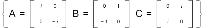
As su(2) is made up of 2 × 2 matrices with entries in ℂ we might be tempted to think that it too needs a basis with eight elements. However there are constraints placed on the make up of su(2)’s basis by the structure of the Lie Algebra. In particular, it can be seen that the elements on the main diagonal are tied together and, as they must be purely imaginary, there is only one component to consider. This means that we only need one basis element to cover the main diagonal, something like:

Equally, the entries on the minor diagonal are also tied to each other. However, this time there is both a real and an imaginary component to consider and so we need two basis elements. We can also note that while the imaginary component is the same for both elements of the minor diagonal, the real components are the negative of each other. So two matrices such as the following will suffice:

We can combine these (and label them) to form a complete basis for su(2) as follows:

Which of course demonstrates that su(2) is of dimension 3. Each of the basis matrices is obviously Skew-Hermitian and with trace zero like all members of su(2).

While the subject of this book is Mathematics, a major motivation lies in Physics and particularly particle Physics. If we multiply each of our three basis vectors for su(2) by – i we get three matrices which are Hermitian rather than Skew Hermitian as follows:

These are known as the Pauli Matrices ^[1], which appear in the Pauli equation, which in turn governs the [non-relativistic] movement of fermions ^[2] in an electromagnetic field. Here I will air some dirty laundry, the only reason why we needed to multiply by – i here is that Physicists like to work with Hermitian matrices, not Skew-Hermitian ones ^[3]. There are actually two whole notations employed in this area, the Mathematics one and the Physics one. They are wholly equivalent, the Physics notation requires a compensating multiplication by – i elsewhere in the overall “machine” to keep things straight ^[4]. Perhaps unsurprisingly, I’ll stick to the Mathematical formulation.

All of which confusion goes to say that I could use my basis for su(2) in an alternative version of the Pauli Equation and the Universe would not bat an eyelid. This is an example of the sometimes all too human aspects of what is often seen as pair of entirely clinical and well-ordered disciplines.

So we have found a use for one of our Lie Algebras in particle Physics, be prepared for more of this stuff. Indeed more is just round the corner, because we are now going to consider su(3).
 
 
su(3)

As explained in a footnote in the last Chapter su(3) is the Real Vector Space of 3 × 3 Skew-Hermitian matrices whose trace is zero, with the Lie Bracket being the commutator.

Similar logic to that which we applied for both u(2) and su(2) in the previous Chapter leads us to conclude that a generic element of su(3) is of the form:

Where a, b ∈ ℝ and α, β, δ ∈ ℂ ^[5].

We can apply the same type of logic that we used to form a basis of su(2) above to come up with the following 8 matrices spanning su(3):

The first three rows above relate to the constraints applied to respectively α, β and δ and are essentially as per the basis of su(2).

The last row recognises that there are two degrees of freedom on the main diagonal, a and b (noting that main diagonal entries are purely imaginary again), but that in each case the trace must be zero.

As was the case with su(2), if you multiply the above basis by – i you create a set of matrices named after an equally eminent Physicist, Murray Gell-Mann. These are as follows:

Readers may question why the scalar 1/√3 has appeared against the last matrix. Well first of all multiplying any basis element by a scalar leaves it still being a basis element, so we could have multiplied by 3,456,323,388,954,407 and still have a basis. Second this term is introduced for technical reasons, which I don’t plan to cover in the main text, but which are briefly alluded to in the notes ^[6].

As with the Pauli Matrices, the eight objects appearing above are all Hermitian and traceless ^[7].

Once more the need for multiplying by – i (and 1/√3) is purely a choice of definitions and the laws of Physics would work fine with the first set of matrices, so long as equations are modified accordingly ^[8].

Again the Gell-Mann matrices are extremely important in particle Physics, this time appearing at the heart of Quantum Chromodynamics and specifically transformations of gluons ^[9], the particles which hold quarks together as part of the strong nuclear force. Again we shall see more of this later.

Before we move on to other matters, let’s quickly look at one more Lie Algebra, u(1).
 
 
u(1)

Looking at our definition of u(2) in Chapter 17, we can see that u(1) is the set of Skew-Hermitian 1 × 1 complex matrices over ℝ with the Lie Bracket again as the commutator. Of course, as we have mentioned before, 1 × 1 matrices are just numbers, however the Skew-Hermitian property still applies to entries on the main diagonal (i.e. the numbers themselves), which leads us to deduce that u(1) is simply the set of purely imaginary numbers, i.e. {ai, a ∈ ℝ}. Clearly u(1) ⊂ u(2) ^[10], so again it suffices to demonstrate closure under vector addition and scalar multiplication to establish that u(1) is a Vector Space.

If a, b ∈ ℝ. then: ai + bi = (a + b)i, which is obviously in u(1)

If a, b ∈ ℝ. then: a(bi) = (ab)i, which is obviously also in u(1)

As multiplication of Complex Numbers is commutative, the commutator is always zero and so fulfils the Lie Bracket properties trivially and we can see that u(1) is also a Lie Algebra. Further we can see that its dimension is one with the obvious basis consisting of {i}.

Note: I wanted to alert readers to a conspiracy theory here, one as far reaching as when Stanley Kubrick helped the US Government to fake the Moon landings. This is encapsulated in the following table: Lie Algebra u(1) su(2) su(3) Dimen-sion 1 3 8 Number of Particles 1 3 8 Particles Photon W+, W–, Z bosons 8 Gluon “colours” Force Electro-magnetic Weak Nuclear Strong Nuclear The Government clearly doesn’t want you to know this information!

We will further examine the connections that the Lie Algebras u(1), su(2) and su(3) have with particle Physics in later Chapters, but we have already established a few linkages here, some direct, some more circumstantial. Next in this Chapter, we will introduce the much trailed and heavily related concept of a Lie Group.
 
 
As Smooth as Silk

Well this should be pretty straightforward. A Lie Group is a Group that is also a differentiable manifold. Oh dear, that is another of my definitions that raises more questions than it answers. A proper treatment of manifolds, let alone differentiable manifolds, is beyond the scope of this book, but I will try to explain these concepts in broad terms. Hopefully I will provide enough of an insight to allow us to move on to other work without getting bogged down in very technical details.

Note: A warning, I am going to be rather non-rigorous here; in the same way that the Pope is rather non-Buddhist. I’m also going to play fast and loose with words, sometimes conflating terms with precise (and different) Mathematical meanings, such as smooth and differentiable, both with each other and with the common-all-garden meaning of smooth. If readers are interested in learning more about these areas without the benefit of my generalisations and hand waving, then I would suggest looking up resources on differential geometry and maybe topology as a good place to start.

Very loosely speaking, a manifold is something that resembles Euclidean space when looked at close-up. Given that most people reading this book will realise that we inhabit the surface of a roughly spherical object (a non-Euclidean space), why does our world seem flat? The answer is that the curvature of the surface of the Earth is such that – at a human scale – it is hard to tell it from a non-curved surface. By extension, an ant may view the surface of a Swiss Ball as flat, or at least flatish, where we perceive it as obviously curved; it is a question of the relative sizes of the observer and the curvature in question ^[11].

This analogy captures the essence of a manifold. Indeed the surface of a sphere (written S²) is an example of a 2D manifold – obviously surfaces have two dimensions. The simplest 2D manifold is a plane, or 2D Euclidean space. One way of saying that the surface of a sphere is a manifold is that it is indistinguishable from a plane if you look at it at a small enough scale relative to the diameter of the sphere. Another example of a non-planar 2D manifold is a torus, what Mathematicians call a smoothed out doughnut shape or quoit; an image of one of these appears at the beginning of this section.

Manifolds can also have dimensions less than two or greater than two. Examples of the first case would include lines (i.e. 1D Euclidean space) and circles (a non-Euclidean 1D space). A counterexample is that a figure of eight is not a 1D manifold; the issue is where the lines cross. A manifold has to resemble Euclidean space close-up everywhere, and the crossing point is an exception to this. An example of a 3D manifold is a 3-sphere (written S³) which is the “surface” of a 4D sphere, i.e. a set of points in a 4D Euclidean space all equidistant from a single point.

So what is a differentiable manifold? Readers may recall differentiation as being one of the two main components of The Calculus. It is the process of determining the gradient of a curve (or a curved surface, or indeed a multidimensional manifold) at a point ^[12]. A differentiable manifold is one that is smooth enough to support differentiation, i.e. the calculation of its gradient (or gradients) at a point.

To take a 1D example, in the diagram above, the curve on the left is smooth and can be differentiated, the curve on the right is jagged and the slope (differential) is undefined where the curve switches back on itself. The formal Mathematical concept of smoothness is not so far removed from what we might think it to be, at least for simple curves and surfaces ^[13].

An alternative way of stating that a manifold is differentiable is that we can establish a tangent to any point in the manifold. For 1D manifolds, this is the meaning of tangent that people recall from geometry, a line touching the curve at a point and with an angle equal to that of the curve at the same point. If we enlarge the left-hand diagram from above then the tangent to the curve at point x = a is something like this:

If we instead think of the 2D manifold S², our spherical surface, then rather than being a line, a tangent at a point is a plane as follows:

Here we can come back to the point we made at the beginning of this section, for the sphere above, as we zoom in, the plane forms a better and better approximation to the surface of the sphere at the point it touches. At least over a small part of space, we can treat spherical geometry as if it was planar geometry, we can linearise it; a concept we will come back to soon. However the immediate objective is to loosely define something called a Tangent Space.
 
 
Going off on a Tangent

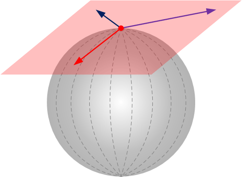
Let’s think of this from a Mechanics point of view in the first instance. Suppose a particle’s movement is confined to S². At any point in time, it will have a direction of travel which is tangential to the surface of S². Therefore it can be seen that – if we describe the particle’s motion by a vector – this vector will instantaneously lie somewhere in the plane tangent to its current position (see the diagram above). Indeed the plane itself can be thought of as consisting of all possible vectors that could describe the particle’s movement at this point. When thought about from this vector-centric point of view, the plane is then called a Tangent Space of the differentiable manifold; a particular type of Vector Space.

What about the situation where the differentiable manifold is also a Group, i.e. the overall structure is a Lie Group? That is an interesting question, but sadly one we cannot answer using the example of S². This is because – for reasons I won’t get into here – S² does not support a Group structure. However something rather like S², but simpler, does, namely S¹ or the circle. Back in Chapter 13 we explored the Group of rotations of a unit circle centred on the origin of either a 2D Euclidean space or the Complex Plane (the two being isomorphic). We found that this formed a Group and, when using the Complex Plane approach, it was the Unitary Group of degree 1, U(1). By way of a refresher:

U(1) = {a + bi, a, b ∈ ℝ and a² + b² = 1}

Or entirely equivalently, the set of Complex Numbers, z, whose complex conjugates are also their inverses, i.e. z z = 1.

The latter definition chimes more with the generic description of the family of Unitary Groups, U(n).

We have already said that a circle is a manifold and it is also clearly a differentiable one (its slope can be calculated by differentiating the equation y = ± √(1 – x²) or by straightforward trigonometry). So this means that U(1) is our first example of a Lie Group. How would we go about constructing its tangent space?

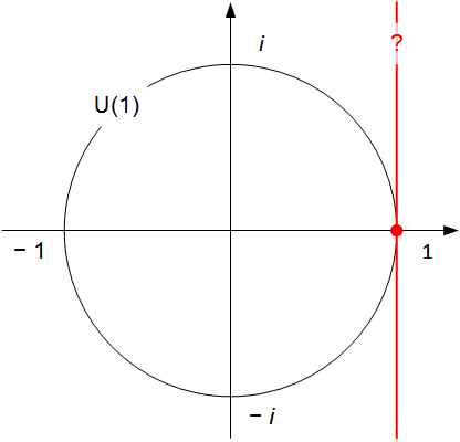
Well a tangent to a circle at a point is always at 90° to a radius ending at the point. If we pick the point 1 (i.e. 1 + 0i) ^[14], which is clearly part of the unit circle, then its tangent is the red vertical line passing through 1 shown above.

Coordinates on this line are the vectors that form part of the Tangent Space. However, we should recall that these vectors are defined with respect to the initial point 1 rather than the origin of our manifold’s coordinate system (the centre of the circle). So we are looking at arrows that start from 1 and go either up or down from it. It can fairly readily be seen with this shift of perspective that the Tangent Space of S¹ at 1 is the set {ai, a ∈ ℝ}, or the purely imaginary numbers.

At this point some bells will be ringing. This set is precisely the one we discovered formed u(1) earlier in this Chapter. Therefore we have determined that the Tangent Space of the Lie Group U(1) at point 1 is the Lie Algebra u(1). At this juncture both our mysterious labelling of Lie Algebras and their connection to Lie Groups is hopefully beginning to become clear. Indeed we can state that:

Every Lie Group defines a Lie Algebra, this is the Tangent Space of the Lie Group at the identity element of the Group ^[15].

Two points: First, we can define a Tangent Space with confidence precisely because the Lie Group must be a differentiable manifold. Second, we can see that our choice of 1 was not accidental as it is indeed the identity element of the Lie Group U(1).
 
 
So we have established a connection between Lie Groups and Lie Algebras and shown a way that the former can lead to the latter. In the next Chapter, we will list some common Lie Groups together with their Lie Algebras and investigate whether or not it is possible to travel the other way; to create a Lie Group from a Lie Algebra. This investigation will involve a refresher on something we have employed more than once already in this book, the exponential function.
 
 

Concepts Introduced in this Chapter Lie Group A Group that is also a differentiable manifold. Manifold Broadly speaking, a structure that is similar to Euclidean space (of whatever dimension is relevant) at each point, but which may be very different from Euclidean space in aggregate. For example the surface of a torus is locally like 2D Euclidean space but a torus is very different to a plane. Differentiable Manifold Again broadly speaking, a manifold which is smooth enough to allow gradients to be calculated at every point, or equivalently tangents to be drawn at every point. Tangent Space An imprecise definition would be the Vector Space consisting of all vectors tangential to a point in a differentiable manifold. Lie Group to Lie Algebra correspondence For a given Lie Group, its Lie Algebra is given by constructing the Tangent Space of the identity element of the Group.

< ρℝεν

|

ℂσητεητs

|

ℕεχτ >

 
Chapter 19 – Notes

[1]	Named after eminent Physicist Wolfgang Pauli.
[2]	Particles with whose spin property is equal to one half. These can be as quotidian as electrons, or the various quarks that make up protons, neutrons and other baryons, or as esoteric as various neutrinos. See the image at the beginning of Chapter 1 for a list, they form the first three columns.
[3]	I’m sure Physicists can – and indeed do – make the same type of comments the other way round about Group Theorists.
[4]	For example in the definition of the commutator. In the next Chapter we will meet the concept of exponentiation, this will also require an additional i using the Physics notation.
[5]	If we set a + b = 0 then the last element of the main diagonal is zero and the 3 × 3 matrix is defined wholly by the top left 2 × 2 entries, which are exactly as for su(2).
[6]	Specifically to ensure that the Frobenius norm of all of the basis elements is the same, √2 in this instance. As the last matrix is the only one to have either more than two non-zero entries or an entry with absolute size different to 1 (|- 1| = |i| = |- i| = 1 of course), it requires adjustment to meet this criteria. In turn this means that, like all of the other Gell-Mann matrices, if we multiply the last one by itself, we get 2.
[7]	Which is another way of saying that their traces are zero.
[8]	The motivation behind things like this can be historical, or it can be to significantly simplify the Physical equations that are being referred to. Any simplification will rear its head in complexity elsewhere, but if equation A is used all the time and becomes simpler, whereas equation B is more seldomly referenced and becomes more complicated, then this may be a logical trade off.
[9]	Actually rotations of gluon fields.
[10]	If we set all the entries save the top left to zero and this to be ai the embedding of u(1) in u(1) becomes evident.
[11]	Determining the extent to which ants have an understanding of Differential Geometry is a very active current research topic.
[12]	For a curve the differential has just one value, for a 2D surface, the differential can vary according to which direction you are travelling; if you follow a river down the valley it has made, the slope will have one set of values, if you climb up the sides of the valley (normally at 90° to the flow of the river), the slope may have another set of values. We will spend some more time looking at differentiation in Chapter 19.
[13]	A more formal definition of smoothness appears in a note box in the next Chapter.
[14]	This point has not exactly been picked at random.
[15]	We will come on to the opposite question, do Lie Algebras determine Lie Groups a bit later on.

Text: © Peter James Thomas 2016-17. Images: © Peter James Thomas 2016-17, unless stated otherwise. Published under a Creative Commons Attribution 4.0 International License.