< ρℝεν

|

ℂσητεητs

|

ℕεχτ >

“Quantum Mechanics is a beautiful generalization of the laws of probability.” – Scott Aaronson

Author’s Note This book is currently a work-in-progress. In case you stumble across it, please note that a number of Chapters are either incomplete or, in some cases, not yet started. The Chapter you are currently viewing falls into these categories. Expect content to be provided here in coming weeks and months.

I have in general eschewed too many comments about the process of writing this book. Glimpses of Symmetry is meant to be a book about Group Theory, not a book about writing a book ^[1]. However, here I am going to make an exception. Has there ever been a book written where the author has not suffered from writers’ block at some point? My guess is there are probably few of these; Glimpses of Symmetry is not an exception to the rule. My specific block was related to Quantum Mechanics. As advertised in the Introduction, this book is primarily about Mathematics, not Physics. However, the motivation behind telling the story that I have been trying to tell is of course Physics-based and relates to explaining the role that Group Theory plays in the Standard Model of Particle Physics. Given this Mathematics / Physics dichotomy, the sort of questions I have got caught up on have been as follows:

Just how much of Quantum Mechanics (and Quantum Field Theory) do I want to include in the text?

• Quite a lot, so that the actual role of is laid bare?
   
• A hand-wavy outline (something common to many a book discussing Quantum Mechanics), which is just about enough of a framework on which to hang the Mathematics?
   
• Or something in between these two extremes?

A factor here is that I am not a Physicist. To do Quantum Mechanics any sort of justice, I would have to devote myself to learning a lot of things that I did not cover in University. The path that I thought was most likely ahead of me is eloquently described by Scott Aaronson as follows:

You start with classical mechanics and electrodynamics, solving lots of gruelling differential equations at every step. Then, you learn about the “black-box paradox” and various strange experimental results, and the great crisis that these things posed for Physics. Next, you learn a complicated patchwork of ideas that physicists invented between 1900 and 1926 to try to make the crisis go away. Then, if you are lucky, after years of study, you finally get around to the central conceptual point: that nature is described not by probabilities (which are always non-negative), but by numbers called amplitudes that can be positive, negative or even complex.

— Quantum Computing Since Democritus – Chapter 9

Scott Aaronson is a theoretical computer scientist and his above-referenced work proved something of an epiphany for me, allowing me to break through my writers’ block and begin the process of finishing this book. The central point that he makes is that, while you can approach learning Quantum Mechanics in the manner he described above, you don’t have to. There is an alternative formulation, in which Quantum Mechanics “falls out” of a process of generalising Probability Theory. This path is essentially a Mathematical one and thus appeals strongly to me. It is Aaronson’s ideas that I will discuss in this Chapter. Just one benefit of his approach (at least speaking selfishly) is that the importance of Unitary matrices appears early on and in a very natural manner. Having acknowledged my considerable debt to Aaronson’s wonderful insight, let’s dive in. Given my desire to make this work as accessible as possible, I’ll start with a basic primer on Probability Theory.
 
 
Chances Are…

Probability Theory relates to the chances of something happening (or not happening). This is probably ^[2] an unsurprising statement. The main concepts in the field are essentially accessible to anyone with experience of placing a bet, or trying to make a decision based on the likelihood of something else occuring. As Probability Theory is part of Mathematics, we need to bring numbers in to the picture. Let’s do this with a rather obvious example before generalising.

Consider that staple of probability exercises, a fair, six-sided die (see some examples above). When this is thrown, there are obviously six things that can happen.

1. We could throw a one
2. We could throw a two
3. We could throw a three
4. We could throw a four
5. We could throw a five
6. We could throw a six

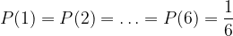
When we say that the die is fair, this means that each of the above is equally likely. Mathematically we call each of the numbers that can be thrown an outcome. We then associate a number, between zero and one, to each outcome which reflects how likely it is to happen; this is called the probability of the outcome. Something with a probability of zero never happens (for example, throwing seven with the above die), something with a probability of one always happens (for example, throwing a number that lies between one and six). Expanding on the second example, if the probability of throwing some number is one and throwing each individual number, say a three, is as likely as throwing any other one, we can then deduce that the probability of throwing a three (or indeed any other individual number), which we denote by , is given by:

One way of thinking about this is to throw the die many times and record both the number of throws and the number of times that, say, three is thrown. We then consider another fraction:

The Law of Large Numbers ^[3] tells us that the more times that we throw the die, the closer that the above fraction gets to the actually probability of throwing a three, which we have already stated is . In the Mathematical language of limits ^[4] we say that:

An example of this appears in the box below:

As Easy as π Instead of throwing a die, let’s consider how often we get a three in another situation, the decimal expansion of everyone’s favourite Irrational Number, . For all intents and purposes, this decimal expansion is essentially a stream of random numbers [5]. Here there are ten possible outcomes, , and if we take it that each is equally likely (see previous footnote), then we should assume that: Let’s look at the frequency with which three appears when we consider different numbers of digits as follows [6]: Number of Digits Number of Threes Frequency of Threes 100 12 0.12 1,000 103 0.103 10,000 1,021 0.1021 100,000 10,026 0.10026 1,000,000 100,230 0.10023 10,000,000 999,965 0.999965 We can see that, as we consider more and more digits, we have: Which is what the Law of Large Numbers tells us will happen.

We can also consider some less obvious outcomes:

We can see that the outcomes with non-zero probability are of these are compound outcomes, made up of our fundamental six outcomes. So

and so on.

We have noted above that the basic outcomes from throwing a fair, six-sided die are each of a one through to a six. We can write the set of possible outcomes as . We have also shown that:

We could also group these probabilities together into a set as follows:

Something that immediately is obvious is that the sum of this set is one. A moment’s thought tells us that this is perfectly natural. The chance of some outcome or other is obviously one, so adding up all the possibilities must also give us one.

Of course we don’t have to have the uniform distribution shown above. Supposing we take some TipEx ^[7] to both the number five and number six on our die, in each case covering up two spots.

Our set of probabilities (for the same six outcomes we had before) now looks like:

We notice again that the sum of the elements remains as one. We are going to come back to this sum later.

Let’s now think about a more general case. Suppose we have a generic event, let’s call it , which has potential outcomes: . Further, let’s assume that the the probability of any one, say , occurring is denoted by . Then value of is a Real Number in the range zero to one. As with our die after we had applied TipEx, the can all be different from each other.

As with the die, if an outcome cannot happen, its probability is assigned the value zero. If it must happen, its probability is assigned a value of one. If the outcome may occur, but is uncertain to do so, then its probability is neither zero, nor one, but somewhere between the two. The closer that a probability P(x_i) is to one, the more likely it is to happen; the closer to zero, the less likely.

We can obviously also gather together these probabilities as follows:

or more simply just write:

Can we say anything about our set ? Well again the sum of this must be one. We can write this as:

To date, we have been considering discrete probabilities, ones where there are a finite number of outcomes, which we can label . We can also deal with continuous probabilities, ones where the outcome of our random variable falls into a continuous range (normally a subset of the Real Numbers). This is covered briefly in the box, we will be mostly dealing with discrete probabilities in this chapter, though it is important to bear the generalisation in mind.

A Lack of Discretion The process is actually somewhat analogous to moving between discrete rotations in the Complex Plane and continuous ones. Things that we covered in Chapters 11 and 13. For a continuous probability distribution, outcomes are denoted by say and their probabilities are given by a function of the outcomes, say . Then will form a curve, perhaps something like the following: With a continuous probability distribution, it doesn’t make sense to talk about the probability of a specific outcome (it will be zero), instead we consider the probability, , that our outcome falls in a range (say between and ) and, instead of a sum, we must use an integral as follows: We can also have that: Which is consistent with our result for discrete probabilities above.

Well that was a bit whistle=stop, in the next section, I’m going to introduce a couple of other concepts that we will need before thinking about generalising what we have established to other number systems. The concepts are of Markov Chains and the Stochastic Matrices that describe them.
 
 
Chain Reactions

I (or more realistically someone else) could write an entire book on this subject, here we are going to just skim the surface.

Let’s start by thinking about a situation that can evolve probabilistically over time. We will start simple and consider a system (it doesn’t matter what at this point) which can start in one of two states, or . Furthermore we have some rules as to how the system can change over time. These might be as follows:

1. If the system is in state , then there is a chance of it flipping to state (and thus of course a chance of it staying in state ).
    
2. If the system is in state , then there is a chance of it flipping to state (and thus of course a chance of it staying in state ).

We can denote the state at a point in time by a pair of numbers, say and . Depending on the field of study, this can be written horizontally or vertically, we are going to adopt the convention of writing them vertically here (this is the approach typically used in Physics). So we have:

If at the start, our system is in state , then this is written:

If it is in state , then this is written:

Once more we note that the sum of the two components is one.

Further, suppose we do not know what the initial state is, absent any other information, it might make sense to say that and are equally likely. We could capture this as:

The above all look rather familiar, right? They look like column vectors don’t they. Well that is just what they are, but we are going to call them probability vectors.

Also, we can write our rule for how the system changes using a rather another familiar device, a matrix, as follows:

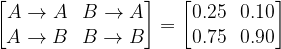
Here note that the sum of any column equals one for reasons that are hopefully obvious from the characteristics of our rules.

Why write our state as something that looks awfully like a vector and our rule for changing state as a matrix? Well so that you can combine the two of course. So maybe we could start with our system in state and see how this then evolves ^[8]:

Rather than being the definitive state () that we started with, we now see that the state of the system is probabilistic, with a 25% chance it is still and a 75% chance that it has become . Applying the matrix has taken us from a determined state to a randomised state.

Let’s take a second step in the evolution of the system (here the input probability vector is the output from the last step):

A third step yields:

In this case, if we keep going we see that:

The interpretation of this is that, in the long run, a system governed by the rules stated up-front will end up in state about 12.8% of the time and state about 88.2% of the time. Or we could say that the potential state of the system is approximately:

We started out with some specific rules here. We could look at things the other way round and ask, what set of matrices (equating to rules for the evolution of the system) are ones that will yield sensible results? We can interpret the last phrase more concretely by saying, that we need matrices which, when applied to a state, lead to a new state whose elements still add up to one (i.e. a probability vector remains a probability vector post transformation). We come to the conclusion that any matrix of the form ^[9]:

where each of are positive Real Numbers, will work. Such matrices are called Stochastic Matrices and they generalise to ones, where all entries are non-negative Real Numbers and each column adds up to one ^[10]. A Stochastic Matrix is one which, when applied to a probability vector, is guaranteed to yield a second probability vector. In general multiplying by a Stochastic Matrix will introduce a random element to a previously definitive state; prior to multiplication, the state was definitively one thing, post multiplication it is (in general) a probabilistic mix of two possible things.

An important thing to note is that if two matrices, and , are both Stochastic, then so are both and ; in particular, will be Stochastic for .

The evolution of the system described by the repetitive application of a Stochastic Matrix is called a Markov Chain. The Markov Chain we worked with above converged to a specific set of values, but this is not always the case. A Chain could instead, for example, cycle round a number of different states (potentially via some intermediate values) in perpetuity ^[11].

It may seem that what we have been doing is rather academic, but Markov Chains have very wide and practical applicability in fields as diverse as meteorology and economics. Famously, Google’s original PageRank algorithm was based on the concept of Markov Chains.

Note: In the earlier sections, we were talking about sets of probabilities of outcomes in a discrete probability distribution, things like: In this section, we have been treating pairs of probabilities as a vector. Let’s stop dissembling and state that we will treat our sets of probabilities of outcomes as a vector as well and – in particular – a column vector such as:

While we have merely scratched the surface of the surface of the surface of Probability Theory here, we are now equipped to consider a generalisation of it.
 
 
Improbable Complexity ^[12]

All the way back in Chapter 7, we considered what would happen if we allowed the question “what is the square root of a negative number?” to be answered. From one point of view, this was wholly counterintuitive as when we square both a positive and a negative number we get a positive one. Surely the square roots of negative numbers can’t exist, can they? Well, as demonstrated in Chapter 7 and many other places in this book, they can exist and lead to beautiful, powerful and entirely practical results.

Here I am going to ask another counterintuitive question, “can a probability be negative?” Indeed why not go the whole hog and instead ask “can a probability be a Complex Number?” Let’s put physical intuition on pause and see where answering this with a “yes” gets us. To avoid disturbing too many people’s equilibrium, let’s drop the visceral word “probability” and refer to our probability-like Complex Numbers as “amplitudes” instead.

Let’s layer another idea on top of this, to date we have been talking about the columns of our probability vectors and of our Stochastic Matrices adding up to one. To be more formal (and recalling some of our language from Chapter 22) “adding up” is equivalent to what is generally called the 1-norm. Very simply put, applying to an -dimensional vector , this is just:

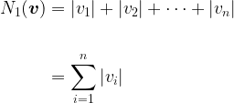
There are other norms, indeed we are very used to the one we are going to adopt here, it’s called the 2-norm, or Euclidean Norm, and arises by applying Pythagoras as follows to the same vector:

So let’s be bold and consider an extension of Probability Theory where positive Real Number probabilities are replaced by Complex Number amplitudes and where the 2-norm of amplitude vectors must add up to one ^[13].

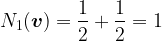
Eschewing dice for the moment, let’s consider something even simpler, the toss of a fair coin, which can come up either heads or tails. The vector (just for kicks, let’s call it ) consisting of the probabilities of the possible outcomes would look like this:

Under our regular 1-norm we have:

However, under the 2-norm we would get:

Which is not what we want, so instead, using the 2-norm, our probability vector for a fair coin is:

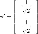
And then:

as we required.

An obvious question would be, what is the equivalent of a Stochastic Matrix in our new and extended Probability Theory? Well – considering the case for the sake of simplicity – we need matrices satisfying:

remembering that each of the letters is a Complex Number.

It can be shown (though I’m not going to do it here) that matrices satisfying the above condition are precisely those whose conjugate transposes are also their inverses. Hopefully readers will recall that these types of matrices have a special name. Yes that’s right, our old friends, Unitary Matrices (see Chapter 13).

Let’s step back here for a second, what have we just stated? Well in regular Probability Theory any operation on a probability vector that yields a second probability vector can be described by a Stochastic Matrix. In our generalisation of Probability Theory to Complex amplitudes and the 2-norm, any operation on an amplitude vector that yields a second amplitude vector can be described by a Unitary Matrix. Maybe this is worth summarising:

Comparison of Probability Theories
Concept	Regular	Generalised
Name of units:	Probability	Amplitude
Units are:	Positive Real Numbers	Complex Numbers
Norm:	1-norm	2-norm
Operations that preserve probability / amplitude vectors:	Stochastic Matrices	Unitary Matrices

 
Of Bras and Kets and Quantum States…

Although clearly I have not demonstrated this in detail above, the generalisation of Probability Theory to amplitudes that are Complex Numbers and use of the 2-norm is perfectly rigorous from a Mathematical point of view. What does this have to do with Quantum Mechanics? Well, as Aaronson points out in his aforementioned book:

Quantum Mechanics is what you inevitably come up with if you start from Probability Theory, and then said, let’s try to generalize it so that the numbers we used to call “probabilities” can be negative numbers. As such, the theory could have been invented by Mathematicians in the nineteenth century without any input from experiment. It wasn’t, but it could have been.

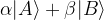
Let’s make things a bit more Quantum Mechanical by introducing some notation due to Paul Dirac, unarguably the greatest British Physicist since Newton. This is a specific way to show probability vectors. Supposing we have the coin-flip situation we saw above when introducing the 2-norm, that is a vector like this:

If we label the outcome where heads is thrown as and that where tails is thrown as , then Dirac’s Ket notation would write the above vector as follows:

The pairing of and is called a “ket” ^[14]. The things that appear within the “ket” are outcomes, the things appearing before the “ket” are amplitudes. It may be somewhat unclear what this notation gets us, but, if we go back to our probability vector for a die with TipEx judiciously applied, i.e.:

We can write this as:

That is we omit the terms with zeros. Note here that the numbers within the kets above are the outcomes (e.g. throw a three) and the numbers before them are (in this case) probabilities (more generally amplitudes).
 
 
…of Double Slits and Things

Let’s use this notation to cover something at the heart of Quantum Mechanics, Quantum Interference.

Before doing this, let’s introduce the most famous example of Quantum Interference, the double-slit experiment. Back in the 1801, Thomas Young created an experiment where a point light source ^[15] is shone through two vertical slits with a screen behind them; the set up is essentially like this:

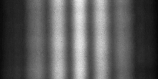
Intuition suggests that rays of light go through the slits, continue on to the screen and create two vertical areas of illumination mirroring the double slits, but rather further apart (see the right-hand end of the above diagram). Indeed, if you cover up one of the double slits, then a single vertical bar of light does indeed appear on the screen, consistent with intuition. However, when Young uncovered the second slit, he observed something different. He saw repeating bands of light and dark appear on the screen. These covered the area between where one might have assumed that two vertical lines would appear and extended out past them as well. The result was something like this:

The classical explanation of this phenomenon relied upon waves. If you throw a pebble into an otherwise calm pool, concentric circles spread out from it in a manner that is immediately familiar.

What happens physically is that the pebble initially pushes some water downwards, the water then rebounds upwards, splashing up to above its previous surface level. This mini column of water then collapses, again pushing the water downwards and the process repeats, gradually dying out. However, as well as being pushed down, the impact of the pebble and the impacts of the following columns of water collapsing also push the water out sideways in all directions. What happens is you get circular waves spreading outwards from the impact site. The peaks and troughs of these mirror the downwards and upwards displacement of water where the pebble hit the surface.

A piece of equipment called a ripple tank reproduces this effect in the lab. Rather than a single pebble, a motor drives a small probe being dipped in and out of the water, creating continuous circular waves. Here is what one looks like:

When two wave generators are used instead, the concentric waves from each overlap. Where the peak from one set of waves meets a trough from the other, the two cancel each other out and the water is calmer than elsewhere. Where instead two peaks meet, the wave is larger than it would be elsewhere. Looking at a ripple tank with this arrangement from above we see:

So the outcome is that we get areas where the wave strength is a minimum (peak + trough), followed by others where it is a maximum (peak + peak), followed by a minimum and so on. Young reasoned that the light in his experiment must be behaving in the same way as the water; that is light must consist of waves.

Under this explanation, light waves emanate from each of the two slits, just as water waves came from both generators in the ripple tank. When a peak from one meets a trough from the other, they cancel each other out (leading to a dark patch; destructive interference). When a peak from one meets a peak from the other, they boost the light level (leading to a light patch; constructive interference). The explanation (and the Mathematics behind it) fitted observations perfectly, so far so good.

But then a number of, previously inexplicable, results began to make Physicists think about alternative interpretations of not just light, but all matter. The era of Quantum Mechanics began to dawn, at first with a faltering light and then with the full glory of the rising sun. This paradigm shift led to an apparent paradox to do with Young’s slits.
 
 
A Quantum Fly in the Ointment

In a quantised view of the world, light comes in discrete, particle-like packets called photons. These can have phases and a stream of photons can thus appear rather wavy ^[16]. Indeed, Young’s experiment can also be explained by streams of photons passing through the slits and subsequently interfering with each other; this yields precisely the same result. If the phase of a photon from slit one is the same as one from slit two, we get constructive interference, if it is opposite, we get destructive interference. So all is still good.

But – there is always a but in the Quantum Realm – here is the thing. If you turn down the light source so that it emits just one photon at a time, then obviously this must go through either slit one or slit two and so there is no possibility of interference. If we use a photographic plate as our screen, each photon will leave a tiny mark and over time these will build up as each successive photon is let through the apparatus. Under this scenario, with interference eliminated, surely we will get the two bright columns predicted; how could anything else happen?

Well this is not what we see experimentally. Despite the fact that only one photon was emitted at a time and – thinking logically – this must have gone through either slit one or slit two, what built up on the photographic plate was an identical series of light and dark bands ^[17]. This is the signature of interference, but – given that one photon was passing through the apparatus at a time – what could it be interfering with?

This is one of the seminal pieces of “quantum weirdness” that is often used to point out just how counterintuitive Quantum Mechanics is. Here are a couple of related explanations:

1. The photon does indeed go through both slits. Indeed it simultaneously takes every possible path between the light source and the screen. This includes a path that loops out of the lab, spins round the Earth a few times, heads to the Sun for a fly-by, comes back to the Earth, into the same lab and hits the screen. It is all of these different paths that interfere with each other and cause the bands of light and dark.

   This explanation emanates from a technique for performing Quantum calculations pioneered by Richard Feynman. In his approach, we integrate over all possible paths that the photon can take. Each path will have a contribution according to how likely it is. So the one looping round the Sun will not have a very big contribution and can be ignored for practical purposes. Whereas Feynman initially proposed this technique purely to aid calculation, he later flirted with it being what is actually happening.
    

2. Up until the point that it actually hits the screen (resulting in a measurement) the photon is not localised. It is not actually a point particle at all, instead it is a wave of probabilities called a waveform, sort of a smeared out cloud. It is the waveform that goes through both slits and it is the waveform that interferes with itself, only to collapse into an actual single outcome when the plate is impinged.

There are other explanations, I have left out the many-worlds interpretation for example. I have never felt terribly comfortable with any of these. Of course the Mathematics just works and we get the right results with impressive precision, but it would be nice to have a better physical interpretation of what is going on. Something that is well less spooky, to borrow Einstein’s word ^[18]. Let’s see if our Generalised Probability Theory, which I am going to start calling Quantum Probability, can help at all.
 
 
????

Note: Here I am closely following a line of argument from both Scott Aaronson’s Quantum Computing since Democritus and from a talk he gave to a High School when still a graduate student back in 2002 [19]. When I contacted him with some questions about QCSD, Scott was kind enough to point me in the direction of the second document himself. In both cases, I have attempted to add some of my own additional explanation. Thus any errors are my fault and not Scott’s.

To show how Quantum Interference can arise naturally from the extension of Probability Theory that we have been studying, let’s consider a Probability Space with just two outcomes, let’s call them and ^[20]. If we consider a state which is definitively , we can write this as (which is of course the same as ). Similarly, another state which is definitively may be written as as (which is the same as ).

Of course we can envisage other, probabilistic states combining some likelihood of both and . If the amplitudes associated with and are respectively and , then our states look like . What can we say about and ?

Well our restriction that the 2-norm must be equal to one gives us:

This is clearly the equation of a circle, which may be visualised as follows:

Any possible state involving a blend of and (known as a mixed state) will then clearly fall on this circle. Equally any transition from one mixed state to another will involve an operation on the original one that leaves the resulting one still on the circle.

[To be completed]
 
 

Concepts Introduced in this Chapter TBC TBC. TBC TBC.

Groups Discovered in this Chapter TBC TBC. TBC TBC.

< ρℝεν

|

ℂσητεητs

|

ℕεχτ >

Chapter 23 – Notes

[1]	An image of an infinite stack of turtles swims unbidden into my mind.
[2]	Irony intended.
[3]	Which is a phrase whose meaning is honoured more in the breach than the observance.
[4]	For more on limits, see both: A section of Chapter 21 and A section of Euler’s Number
[5]	Whether or not the full decimal expansion of behaves like a stream of random numbers is, perhaps surprisingly, an open question. You can read about the details in a section of my article, The Irrational Ratio. However, a statistical analysis of the first few trillion digits of suggest that this is indeed the case. While not conclusive proof of the stronger result, it is enough for me to rely on the much smaller number of digits I use in my example.
[6]	Here I am relying upon a helpful page that has calculated the frequency with which different digits appear in .
[7]	Wite-Out.
[8]	We pre-multiply the vector by the matrix. If we had chosen to write our state vector horizontally, we would post-multiply instead.
[9]	It is quite typical to write these in the equivalent form of:
[10]	Actually, this is a Left Stochastic Matrix, one where the rows all sum to one is called a Right Stochastic Matrix; one where both rows and columns sum to one is called a Doubly Stochastic Matrix.
[11]	Any Markov Chain that is not periodic and also irreducible will converge. Saying more than this is beyond the scope of this book.
[12]	Not to be confused with Irreducible Complexity. If you look this term up, you will see it is synonymous with “hogwash”.
[13]	We should also allow our amplitude vectors to be infinite in size, but you can do this in normal Probability Theory, it’s equivalently the continuous distributions we covered briefly in a box.
[14]	This slightly odd terminology arises from the word “bracket”. There is a sister expression to the “ket”, namely the “bra”, written , which covers the first part of the word. Combining them, we get a “bra-ket”, , which is actually a fancy way of writing an inner product. We won’t be worrying about “bra”s here.
[15]	It is obviously a linear light source, but looks like a point from above which is the perspective of the schematics included here.
[16]	I am playing rather fast and loose with the concept of phase here, but as this is the way that many Physicists habitually approach Mathematics, I feel somewhat justified.
[17]	The original experiment used electrons, not photons. The results were the same and have since been reproduced with photons as well.
[18]	Einstein was talking about Quantum Entanglement, or “spooky action at a distance” as he termed it, but the observation applies here as well.
[19]	See: Quantum Computing for High School Students.
[20]	Perhaps we would like to make these more concrete, maybe we are talking about a photon here and some property of it, which can be either one value or another, perhaps up and down spin angular momentum; but the physical realisation is not material to the argument.

Text: © Peter James Thomas 2016-18. Images: © Peter James Thomas 2016-18, unless stated otherwise. Published under a Creative Commons Attribution 4.0 International License.